Troubleshooting High Latency in Real-Time Genomic Analysis
By Dr. Zubair Khalid, DVM, MS, PhD ·

Real-time genomic analysis means the computational pipeline keeps pace with the sequencing instrument. Reads flow off the machine continuously, and the analysis result, whether that is a metagenomic profile, a pathogen identification, or a coverage track, is expected to appear minutes after the data, not days. When that gap grows, the analysis has a latency problem.
The most likely cause, in the majority of cases, is not the alignment algorithm or the compute engine. It is the pipeline waiting on data. Reads are being produced faster than they are being transferred, staged, partitioned, or handed to the analysis engine, and the expensive compute resources you are paying for sit idle between batches. The first thing to check is the timestamp gap: compare the time a read chunk was written by the instrument with the time the first stage of your pipeline actually processed it. If that gap accounts for most of your end-to-end delay, you have an ingestion problem, and everything downstream is a symptom rather than a cause.
This guide walks through the causes of high latency in real-time genomic analysis from the most common to the rarest, explains the mechanism behind each failure, gives you a diagnostic sequence you can follow, and closes with prevention practices. The focus is on cloud bioinformatics, particularly pipelines built on AWS and on Apache Spark, because that is where most real-time genomics runs today.
Start Here: The Two-Minute Triage
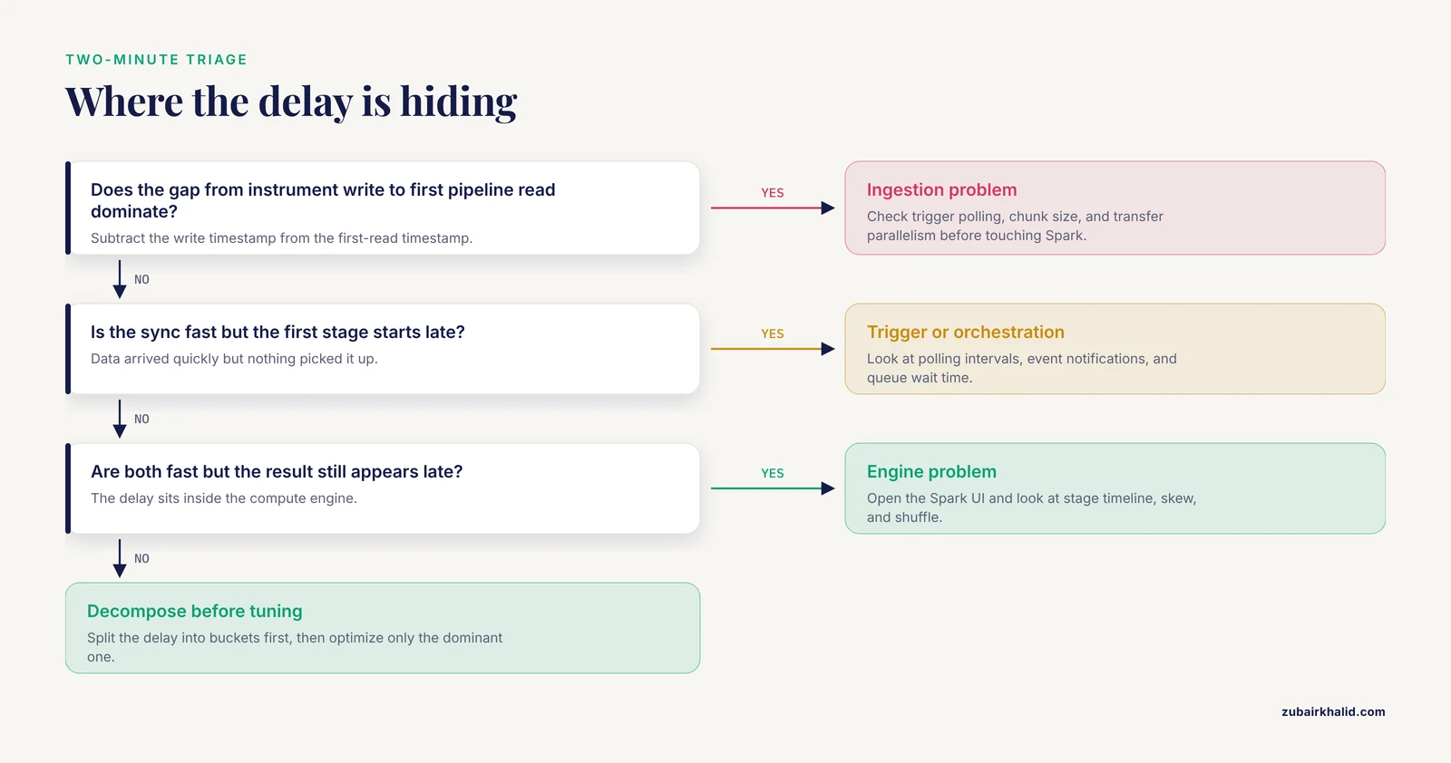
Before you touch a single configuration setting, answer three questions with timestamps.
- When did the sequencer finish writing the chunk of reads?
- When did your pipeline first read that chunk?
- When did the final result for that chunk appear?
Subtract the first from the second. That is ingestion latency. Subtract the second from the third. That is processing latency. Almost every latency incident falls heavily into one of those two buckets, and knowing which bucket you are in saves hours of misdirected debugging.
A fast way to collect these timestamps is to log them at each pipeline boundary. For example, a wrapper script around an S3 transfer can record the wall clock before and after:
date +%s.%N
aws s3 sync /data/flowcell/run42/ s3://genomics-raw/run42/
date +%s.%N
If the sync step takes most of the budget, stop optimizing Spark. If the sync is fast but the first processing stage starts late, you have a trigger or orchestration problem. If both are fast but the result still appears late, the delay is inside the compute engine, and that is where the deeper sections of this article apply.
Why Latency Matters in Real-Time Genomic Analysis
Real-time genomics differs from batch genomics in one fundamental way: the value of the result decays with time. A clinical metagenomics result that arrives after the sample has already been treated is worth less than one that arrives during the same shift. A surveillance signal that surfaces a week after sequencing is a historical record, not an alert. The engineering goal is therefore low end-to-end latency, measured from the moment reads leave the instrument to the moment a usable result is in front of a human.
Latency has several components, and they add up:
- Instrument time to first data. How long after the run starts before usable read chunks exist.
- Transfer time. Moving basecalls or FASTQ/BAM data from the instrument or local server to cloud storage.
- Trigger and scheduling time. How long the pipeline waits before it notices new data and starts work.
- Queueing time. Time spent waiting for compute capacity, licenses, or a job slot.
- Processing time. Actual compute: alignment, profiling, variant calling, aggregation.
- Result delivery time. Writing outputs, updating a dashboard, notifying a user.
Each component can hide a different failure. The most common mistake in real-time genomics latency troubleshooting is optimizing the component that is easiest to measure, usually processing time, when the dominant delay sits in transfer or scheduling.
Real-Time Genomics Latency Troubleshooting Causes at a Glance
The table below is the core of this article. Work through it top to bottom, because the rows are ordered from most to least common.
| Symptom | Likely cause | How to confirm | Fix |
|---|---|---|---|
| Compute nodes idle, then burst into work every few minutes | Batch-oriented trigger, large file chunks, or cron-based polling | Compare instrument write timestamps with pipeline start timestamps | Switch to event-driven triggers such as S3 event notifications, reduce chunk size |
| Sync or upload step dominates the timeline | Insufficient upload bandwidth, single-threaded transfer, TLS handshake overhead per file | Time the transfer step directly, check network throughput from the instrument host | Use multipart and parallel transfer, aggregate small files, upgrade the instrument-side link |
| Pipeline fast on small runs, slow on large ones | Reference database too large for the memory and partition layout | Watch memory pressure and shuffle volume as reference size grows | Partition the reference, use compressed or indexed reference structures, scale out nodes |
| A few tasks in every Spark stage run much longer than the rest | Data skew or straggler nodes | Look at the Spark stage timeline, sort tasks by duration | Repartition on a higher-cardinality key, salt skewed keys, replace slow nodes |
| Every stage takes about as long as the shuffle write | Shuffle-heavy design, too few or too many partitions | Check shuffle read and write volumes in the Spark UI | Tune partition counts, cache reused intermediate data, reduce shuffle via broadcast joins |
| Latency spikes at fixed intervals | Autoscaling cold starts or spot instance reclamation | Correlate latency with cluster scale-up events in cloud monitoring | Keep a warm minimum cluster, prefer on-demand capacity for the latency-critical path |
| Results correct but consistently minutes late | Queueing behind batch jobs or other tenants | Inspect queue times in the scheduler or job manager | Isolate the streaming lane, reserve capacity, prioritize streaming jobs |
| Latency grows steadily over a long run | Memory leaks, garbage collection pressure, growing state | Watch JVM GC logs and memory graphs over hours | Restart long-lived executors, fix state growth, right-size executor memory |
| High latency only from certain networks or sites | Path MTU issues, DNS delays, proxy overhead | Test with path MTU discovery tools, time DNS resolution | Fix MTU or VPN configuration, cache DNS, use private connectivity |
Cause 1: Data Ingestion Bottlenecks, the Most Common Failure
In cloud bioinformatics, the sequencing instrument almost never talks to the compute cluster directly. Data lands in an object store such as Amazon S3, and the pipeline is triggered by the arrival of new objects. Every hop in that path can add latency.
Mechanism. Modern sequencers emit data continuously, but many pipelines still process it in large, periodic chunks. If your trigger fires only when a full lane, a full tile, or a full hour of data is complete, you have imposed a floor on latency that no amount of compute tuning can remove. On top of that floor, single-threaded transfers, small-file overhead, and slow instrument-site links each add delay.
How to confirm. Log the arrival time of every object in your raw-data prefix and compare it with the time the instrument wrote the corresponding file. CloudWatch S3 metrics, or a simple Lambda function on S3 event notifications that writes arrival timestamps, will show you the true ingestion lag distribution.
How to fix.
- Move from polling to event-driven triggers. An S3 event notification writing to SQS, which in turn starts your processing job, removes the polling interval entirely.
- Reduce the unit of work. If you currently process per-hour FASTQ dumps, switch to per-chunk processing so each analysis increment is small and predictable.
- Aggregate small files before heavy processing. Thousands of tiny objects create per-request overhead in object stores. Concatenate or pack small chunks into larger objects at the ingestion boundary, then split them into analysis-sized partitions inside the pipeline.
- Parallelize the transfer. Tools such as
aws s3 syncalready use multipart transfers for large files, but a directory of many small files benefits from running several sync operations concurrently.
Cause 2: Storage and Object-Store I/O Patterns
Even after data arrives in the cloud, the way the pipeline reads it can dominate latency.
Mechanism. Object stores are optimized for large, sequential, concurrent reads. A distributed alignment job that has each of sixty-four executors perform hundreds of small GET requests against the same prefix can saturate per-prefix request rates and suffer retries. Similarly, a pipeline that writes many small intermediate files between stages pays the write and read cost four or five times over.
How to confirm. In CloudWatch, look at S3 request metrics for your bucket, filtered by prefix. High rates of throttling-related errors, or request latencies in the hundreds of milliseconds during pipeline runs, indicate I/O pressure. Inside Spark, the task-level input metrics in the Spark UI show how much data each task actually read and how long it waited.
How to fix.
- Layout matters. Store input data partitioned the way the pipeline consumes it, for example by run and chunk, so each executor reads a contiguous object rather than scanning a listing.
- Use S3 Transfer Acceleration or a gateway only where the transfer path, not the pipeline, is the bottleneck. For compute inside the same region as the bucket, region-local reads are already fast and acceleration adds nothing.
- Keep intermediates in memory or on local instance storage where the data is reused. In Spark, persisting an intermediate DataFrame that is used by two downstream stages can halve the per-chunk processing time.
- Watch for metadata-heavy patterns. Listing a prefix with tens of thousands of objects before every chunk adds seconds to minutes of pure overhead per cycle.
Cause 3: Undersized or Slowly Provisioned Compute
This is the category where AWS genomics architecture decisions show up most clearly in latency numbers.
Mechanism. Cloud compute is elastic, but elasticity has a cost in time. When a cluster scales up from zero or from a small baseline, instance launch, image pull, node bootstrap, and executor registration together take minutes. If your pipeline scales up on demand for each chunk, every chunk pays that startup tax. Spot instances make this worse in a different way: a two-minute reclamation in the middle of a stage costs you the entire stage and a re-execution.
How to confirm. Correlate your latency time series with cluster provisioning events. In Amazon EMR, instance group and instance fleet events are logged and visible in the console and through the EMR API. In the Spark UI, the executors tab shows when each executor registered relative to job start. If the first task of a stage waits for executors that have not finished launching, you have found your delay.
How to fix.
- Keep a warm minimum cluster sized for your steady-state streaming load. Scale out only for burst absorption, not for baseline capacity.
- On Amazon EMR, enable managed scaling with a sensible minimum capacity, and use instance fleets so the service can pick any matching instance type from several families rather than waiting for one specific type.
- Put the latency-critical streaming lane on on-demand capacity. Spot is excellent for batch pre-processing, index building, and reprocessing, but a spot reclamation in a real-time path converts directly into a latency spike.
- Pre-bake your environment into a custom AMI or a pre-pulled container image so node bootstrap does not download dependencies at launch time.
Cause 4: Distributed Framework Misconfiguration in Spark
Many real-time genomics pipelines are built on Apache Spark because it provides parallel processing and a streaming architecture in a single framework. Flint, a metagenomics profiling pipeline built on Spark for fast real-time profiling of samples against large reference collections, is a good example of this design pattern, and it demonstrates both the power of the approach and the tuning discipline it requires [1]. On Amazon EMR, Flint profiled one million Illumina paired-end reads against a reference collection of more than 43,000 bacterial genomes in 67 seconds on 64 machines, an order of magnitude faster than the state of the art at the time while using a much larger reference collection [1]. That kind of performance does not come from Spark by default. It comes from correct parallelism.
Mechanism. Spark divides work into stages separated by shuffles, the all-to-all data exchanges that occur when records must be regrouped, for example by reference genome or by sample. Three misconfigurations dominate latency in this setting:
- Wrong partition count. Too few partitions leave cores idle. Too many partitions drown the scheduler in task overhead, which is measured in milliseconds per task but adds up across thousands of tasks per chunk.
- Data skew. If reads are partitioned by a key that groups unevenly, for example by barcode when one barcode holds most of the data, one task does most of the work and the stage waits for that single straggler.
- Unnecessary shuffles. Every avoidable shuffle adds network transfer, serialization, and disk I/O. A join against a small lookup table implemented as a shuffle join instead of a broadcast join is a classic example.
How to confirm. Open the Spark UI during a live run. Look at three things:
- The stage timeline. Gaps between stages mean scheduling or dependency overhead. One long task at the end of an otherwise fast stage means skew.
- The shuffle read and write volumes per stage. If a stage that does trivial work shows heavy shuffle, the plan is wrong.
- The executor summary. Cores that are idle while other executors are saturated confirm either skew or a partition count mismatch.
How to fix.
# Example Spark session tuning for a streaming genomics job
spark.conf.set("spark.sql.shuffle.partitions", "512")
spark.conf.set("spark.default.parallelism", "512")
spark.conf.set("spark.network.timeout", "600s")
spark.conf.set("spark.executor.heartbeatInterval", "60s")
The right partition count depends on your data volume per chunk and your cluster shape. A practical starting heuristic is two to four tasks per available core per stage, then adjust from observation. For skew, repartition on a higher-cardinality key or add artificial key salting to split a hot key across several tasks. For avoidable shuffles, broadcast small reference or metadata tables and cache any intermediate that more than one stage consumes.
Cause 5: Reference Database Scale and Index Design
The size of your reference collection is a direct input to per-read processing cost, and it interacts strongly with memory.
Mechanism. Alignment and profiling tools build some index over the reference collection, and the query cost per read scales with the index design. Tools designed for a small representative set of genomes degrade when pointed at large collections, both because the index grows and because lookups hit more candidate targets per read. The Flint authors made this observation explicitly: existing profiling tools do not scale well to large reference genome collections, yet larger collections give a more complete and accurate picture of the bacterial population in a sample [1]. Their solution was to treat the reference search as a big data problem, exploiting Spark's parallelism to map reads against a reference collection of 43,552 bacterial genomes totaling about 170 GB [1].
How to confirm. Run your pipeline against reference collections of increasing size on a fixed cluster and record per-chunk processing time. If processing time grows faster than linearly with reference size, your tool or index design is the bottleneck, not your cluster.
How to fix.
- Choose tools designed for large reference collections. A tool whose authors demonstrate scaling to tens of thousands of genomes on a distributed framework will behave very differently from a tool designed for a few hundred [1].
- Partition the reference across the cluster so each executor handles a slice, and parallelize read queries against all slices simultaneously. This is the core of the Spark-based approach.
- Keep the reference index in memory. Spilling a large index to disk per stage turns a compute problem into an I/O problem.
- Curate the reference set deliberately. Removing redundant or low-quality genomes from the collection reduces index size without reducing the biological coverage that matters for your application.
Cause 6: Queueing, Scheduling, and Batch Habits Inside a Streaming Pipeline
Latency problems often survive every infrastructure fix because the workflow manager was designed for batch thinking.
Mechanism. A batch workflow engine typically runs steps in a fixed sequence and waits for each step to complete across the whole dataset. In a streaming context this serializes chunks behind each other and behind unrelated batch work. A nightly reprocessing job or a colleague's large cohort analysis on the same queue can add minutes of waiting to every real-time chunk.
How to confirm. Most workflow engines and job schedulers expose queue time per job. Compare queue time with run time. If queue time is a large fraction of total latency, scheduling is the problem, and no amount of code optimization will help.
How to fix.
- Separate the streaming lane from batch work at the queue, cluster, or account level. In AWS terms, distinct EMR clusters, or distinct Amazon EC2 purchase options and capacity reservations, keep batch load from taxing the real-time path.
- Configure job priority so streaming jobs preempt or outrank batch jobs where the scheduler supports it.
- Convert whole-file batch steps into per-chunk streaming steps where the algorithm allows it. Aggregation steps that require complete data are the exception, and they define the minimum possible latency for those outputs.
Cause 7: Rare and Environmental Causes
When the common causes are excluded, work through these less frequent ones.
Garbage collection and JVM pressure. Long-running Spark executors accumulating state can develop GC pauses that appear as random per-task stalls. GC logs will show pause durations. The fix is tuning executor memory and overhead, or periodically recycling executors, which Spark supports natively through executor restart policies.
Network path problems. Latency that appears only from certain sites, or that fluctuates with time of day, points to the network path. Path MTU mismatches, VPN concentrator load, and DNS resolution delays are the usual suspects. Path MTU discovery tools and DNS timing checks isolate these quickly. On AWS, traffic between VPCs in the same region over the backbone is fast, while traffic through a misconfigured NAT gateway or a peering path can be noticeably slower.
Instrument-side delays. Sometimes the pipeline is blameless and the instrument's own basecalling or export step is the delay. Check the instrument's export logs and its local storage fill level. A nearly full local disk on the instrument host slows writes and can back up the export process.
Container image pulls. If each chunk launch pulls container images from a remote registry, tens of seconds to minutes vanish per launch. Pre-pull images on node bootstrap, or host images in a registry inside the same region.
Cold caches and cold JIT. The first chunk after a cluster restart always runs slower as JIT compilation and caches warm up. Benchmark steady-state performance, not first-chunk performance.
A short safety note on debugging network problems: resist the urge to open security group ports to the internet or disable TLS verification to "make debugging easier." Genomic data, particularly human sequence data, is identifiable information, and a misconfigured security group can expose it. Diagnose network issues from inside the VPC with proper IAM-scoped credentials, and keep encryption on at every hop.
A Diagnostic Sequence You Can Follow
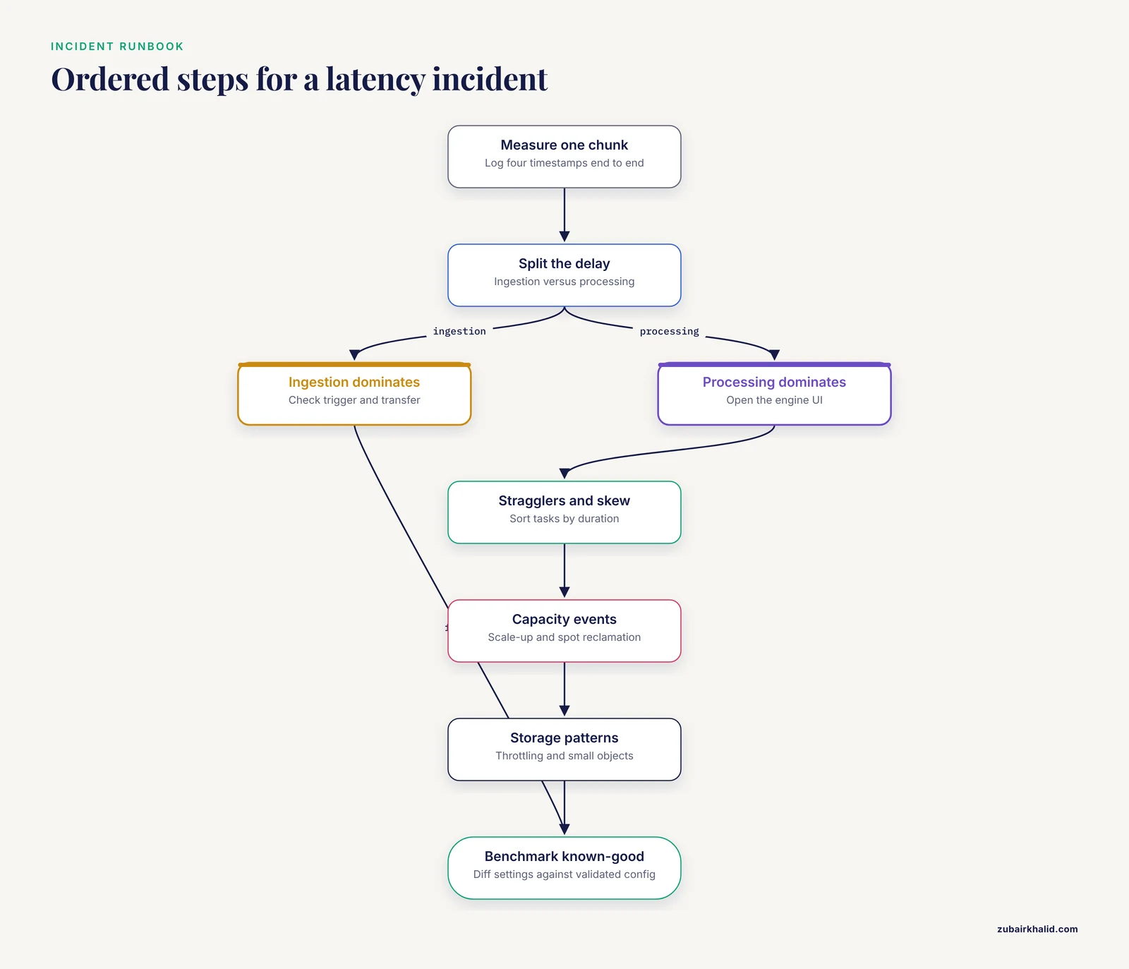
When an incident happens, this ordered sequence resolves the overwhelming majority of cases without guesswork.
- Measure the end-to-end latency for one chunk. Instrument write time, data arrival time in the cloud, pipeline start time, per-stage durations, result publication time.
- Split the delay into ingestion and processing. The two-minute triage at the top of this article does this.
- If ingestion dominates, examine the trigger. Polling intervals, chunk size, transfer parallelism, and instrument-side export are the usual findings.
- If processing dominates, open the engine's UI. For Spark, the stage timeline, task duration distribution, shuffle volumes, and executor summary answer most questions.
- Look for stragglers and skew first. One slow task per stage is the single most common in-engine finding.
- Check for capacity events. Scale-up delays, spot reclamation, and queue contention correlate strongly with latency spikes.
- Check storage patterns. Request throttling, excessive small objects, and repeated reads of the same data.
- Benchmark against a known-good configuration. Re-run a fixed, representative chunk against a configuration you have previously validated, and diff the settings.
Monitoring That Catches Latency Early
Prevention starts with measurement. The minimum monitoring set for a real-time genomics pipeline:
- End-to-end latency per chunk, exported as a metric from your orchestrator. This is the headline number and the only one stakeholders care about.
- Per-stage processing times from the compute engine, so regressions localize to a stage rather than a mystery.
- Ingestion lag, the difference between instrument write time and cloud arrival time.
- Cluster capacity and provisioning events, including scale-up actions and spot interruptions.
- Storage request metrics, including throttling errors and request latency on the prefixes the pipeline touches.
Alert on the trend, not the spike. A single slow chunk usually has a mundane explanation. A steadily rising p95 latency over days means something is degrading, and finding it before it becomes an incident is the entire point of monitoring.
Prevention Practices
Pipelines that stay fast share the same habits.
Design for streaming from the start. Event-driven triggers, small chunks, and stateless per-chunk processing. Retrofitting streaming onto a batch architecture is harder than building it correctly.
Validate scale before you need it. The Flint benchmark, one million paired-end reads against more than 43,000 genomes in 67 seconds on 64 machines, exists because the authors measured their pipeline at scale and designed the parallelism around the reference collection [1]. Run your own benchmark at your real data volume and your real reference size, and re-run it whenever either changes materially.
Keep the latency-critical path dedicated. Separate clusters, queues, or accounts for streaming versus batch. Cross-contamination between the two is a chronic source of unexplained latency.
Pin and pre-stage dependencies. Custom AMIs, pre-pulled container images, and versioned reference indices mean a scale-up event adds compute capacity without adding setup time.
Re-benchmark after every meaningful change. A new reference build, a tool upgrade, or a change in read length all shift the performance envelope. A ten-minute benchmark on a fixed test chunk catches regressions before production does.
Document the expected timeline. Write down the normal latency for each component of one chunk. When numbers drift, you will know immediately which component moved.
Common Mistakes and Limitations
These are the errors that show up repeatedly in real-world latency investigations.
- Optimizing the wrong component. Teams tune alignment parameters for days while the trigger polls every fifteen minutes. Always decompose the end-to-end latency before optimizing anything.
- Benchmarking first-chunk performance. Cold caches, cold JIT, and cold nodes make the first chunk after restart unrepresentative. Measure steady state.
- Confusing throughput with latency. A pipeline that processes a million reads per minute in aggregate can still have terrible per-chunk latency if chunks queue behind each other. Report both numbers separately.
- Treating autoscaling as free. Every scale-from-low event pays node startup. A warm minimum cluster is usually cheaper in both latency and, for streaming workloads, overall efficiency.
- Ignoring data skew because averages look fine. Mean task duration hides the single straggler that defines stage completion time. Look at the distribution.
- Letting batch jobs share the streaming path. A shared queue turns every large batch submission into a latency incident.
- Assuming a larger reference collection must mean proportionally slower analysis. With the right parallel architecture, large collections are tractable, and their biological payoff in profiling accuracy is the reason to use them [1]. The scaling behavior depends on the tool design, not just the size.
- Changing many parameters at once. When tuning, change one setting, re-benchmark, and record the result. Simultaneous changes make causation impossible to assign.
One limitation deserves an honest statement. Published benchmarks, including the Flint results cited here, reflect specific reference collections, read types, and cluster configurations [1]. Your numbers will differ. Use published results to set expectations for the order of magnitude and the design principles, then measure your own pipeline on your own data. And a note on scope: this article addresses computational infrastructure. Individual analytical results, particularly clinical ones, always require domain-expert interpretation, and this article does not replace it.
Frequently Asked Questions
What counts as high latency in real-time genomic analysis?
There is no universal threshold, because acceptable latency depends on the application. A surveillance dashboard may tolerate hours while an intra-outbreak pathogen typing workflow may require results within minutes of read production. Define your own latency budget per application, measure end-to-end latency per chunk against it, and treat any sustained excursion above budget as an incident worth investigating.
What is the most common cause of latency in cloud bioinformatics pipelines?
Data movement and scheduling, not compute. Pipelines that poll for new data, process in large chunks, or scale compute up from a low baseline spend most of their wall-clock time waiting. Event-driven triggers, smaller processing chunks, and a warm minimum cluster remove the majority of this delay in most architectures.
How do I tell whether latency comes from compute or from data transfer?
Timestamp the same chunk at four points: when the instrument wrote it, when it arrived in cloud storage, when the pipeline started processing it, and when the result was published. The gaps between consecutive timestamps assign the delay to ingestion, queueing, processing, or delivery. This four-timestamp decomposition resolves most incidents in minutes.
How does Apache Spark affect real-time genomics latency?
Spark gives you distributed parallelism and a streaming architecture, which is why pipelines such as Flint use it for fast metagenomic profiling against large reference collections [1]. But default Spark configurations are rarely optimal for genomics workloads. Partition counts, shuffle behavior, and data skew determine whether you get Spark's documented performance or a fraction of it. The Spark UI is the primary diagnostic tool.
Does a bigger reference genome database always make analysis slower?
Not proportionally, and not necessarily at all. Tools designed for small reference collections degrade badly as the collection grows, but distributed tools that partition the reference across a cluster keep per-chunk processing fast even against collections of tens of thousands of genomes. Flint mapped reads against a 170 GB collection of 43,552 genomes in 67 seconds on 64 machines [1]. The tool architecture matters more than the collection size.
Can AWS genomics services like Amazon EMR support streaming analysis?
Yes. Amazon EMR runs Spark Structured Streaming and related frameworks, and the Flint pipeline was demonstrated running on Amazon EMR for real-time metagenomic profiling [1]. The requirements are a warm minimum cluster for latency-sensitive work, event-driven ingestion from S3, and Spark configuration tuned for your chunk size and cluster shape.
Should I use spot instances for latency-sensitive genomic workloads?
Generally no, not on the latency-critical path. Spot capacity is significantly cheaper but can be reclaimed with little warning, and a reclamation mid-stage costs the stage plus a re-execution. Use spot for batch pre-processing, index building, and reprocessing, and use on-demand capacity or reservations for the streaming lane where consistent latency is the product.
How often should I benchmark my real-time genomics pipeline?
Benchmark on every meaningful change: a new reference build, a tool or framework upgrade, a change in read length or data volume, or any cluster topology change. A fixed, representative test chunk with recorded per-stage timings takes minutes to run and catches regressions that would otherwise surface as production incidents. Re-benchmarking after changes is the single highest-value prevention practice in this domain.