How to Choose an R Package for Large Genomic Data
By Dr. Zubair Khalid, DVM, MS, PhD ·

Two R packages can run the same statistical test and return the same numbers, yet one finishes overnight on your workstation while the other crashes halfway through loading the file. That difference is memory strategy and engineering, not statistics, and it is the single most important thing to compare when you pick an R package for large genomic data. The rule of thumb is simple. Match the package's memory strategy to the size of your data, check that it parallelizes on the hardware you actually have, and then benchmark it on a slice of your own data before you commit weeks of analysis to it.
This guide walks through the real comparison criteria, lays out the main options side by side with their pros and cons, and works through concrete scenarios from proteomics, methylation, GWAS, and genomic prediction so you can map them onto your own project.
R for bioinformatics, and where it hits a wall
R is the default interactive language for genomics for good reasons. Bioconductor provides standardized data containers for ranges, assays, and experiments, and thousands of peer-reviewed packages sit on top of them. Most published genomic methods ship with R code, so reproducing a paper usually means opening R first.
The wall appears at scale. R keeps objects in RAM, and a typical analysis server has tens to a few hundred gigabytes of it. Whole-genome assays blow past that quickly. A bisulfite sequencing pipeline built around the R/Bioconductor package scmeth was designed for whole-genome datasets with more than 100 GB of raw data per sample and for single-cell methylation datasets with thousands of cells, which tells you where ordinary data frames stop working [1]. The same pressure shows up in statistical genomics. The BESSiE software was written specifically because script based environments like R may not handle large-scale genomic marker data or exploit model properties that save computing time and RAM when fitting Bayesian mixed models [2].
The practical consequence is that "large" is not one problem. A 50-sample RNA-seq count matrix, a 10,000-sample DIA proteomics experiment, and a biobank-scale genotype file each stress a different part of the pipeline. Your comparison of r package large genomic data comparison options should start by classifying your bottleneck.
A five-question framework for choosing
Before looking at any package name, answer these five questions. They determine which pros and cons actually matter for your project.
1. Can the data fit in memory, and what happens if it cannot?
Estimate your object sizes honestly. A matrix of 1 million features by 1,000 samples stored as doubles is about 8 GB before any copies, and R copies aggressively during transformations. If your data fits comfortably, an in-memory package is usually the fastest and simplest choice. If it does not, you need a package with an explicit out-of-memory strategy, such as file-backed arrays, chunked processing, or a companion package built for big data. MSstats, for example, has a companion package called MSstatsBig designed for DIA mass spectrometry datasets too large to fit into a standard computer's memory [3]. Choosing a purely in-memory package for data that exceeds RAM is the most common and most expensive mistake in this space.
2. Does the package parallelize, and on what hardware?
Scale is not only about memory. Check whether the package supports parallel backends, and whether those backends match your infrastructure. Some packages parallelize across loci or individuals, which maps naturally onto cluster nodes. The gghybrid package treats each individual and each locus as an independent analysis, making it highly parallelizable for Bayesian hybrid index and genomic cline estimation on both small and large biallelic datasets [4]. Other packages parallelize across chunks of a matrix, which works well on a single multicore machine but needs adaptation for a scheduler-driven cluster. A package that is single-threaded and in-memory can be perfectly adequate for a thousand samples and unusable for a hundred thousand.
3. Does the ecosystem fit your problem?
R for bioinformatics is not a monolith. Bioconductor packages share data containers, which makes them composable. A scmeth QC step feeds naturally into downstream methylation analysis because both live in the same data model [1]. Domain-specific packages outside Bioconductor often accept simpler input formats but expect you to build the glue yourself. Standalone engines such as BESSiE, which is parameter file driven and command line operated, sit outside R entirely and are best treated as calculators you call from an R script [2]. The right choice depends on how much of your workflow you want to live inside one ecosystem.
4. Is it maintained, tested, and reproducible?
Large analyses run for months, so the package needs to survive that period. Look for Bioconductor release cycles, a Docker image, a versioned manual, or an archived release. The MethylMasteR framework deliberately deployed its comparison of four methylation-based CNV calling algorithms as a single R package inside a Docker image, precisely so the comparison could be standardized and rerun [5]. A package that ships with a container you can pull today will still produce the same result two years from now. A package installed from a moving development branch will not.
5. Is there benchmark evidence, and on data shaped like yours?
Method papers and package vignettes frequently report benchmarks. Read them critically. PRSice-2 was shown to be dramatically faster and more memory-efficient than PRSice-1 and alternative PRS software such as LDpred and lassosum, while maintaining comparable predictive power on biobank-scale data [6]. That is exactly the kind of evidence you want, because it was measured at the scale the tool targets. A benchmark on a 20-sample toy dataset tells you little about behavior at 20,000 samples, because scaling behavior, not single-core speed, is what changes.
Side-by-side comparison
The table below organizes the strongest-known options by strategy rather than by field, because strategy is what you are actually choosing.
| Option | Type | Scale strategy | Pros | Cons | Best for |
|---|---|---|---|---|---|
| Bioconductor core infrastructure (GenomicRanges, SummarizedExperiment, HDF5Array-style file-backed classes) | R/Bioconductor | File-backed arrays, standardized containers | Composable, reproducible, huge ecosystem | You must assemble the workflow yourself | Building any large genomics workflow from parts |
| MSstats plus MSstatsBig | R companion packages | Big-data companion for out-of-memory processing | Same statistical model across small and huge DIA experiments | Proteomics-specific model assumptions | DIA proteomics beyond standard RAM [3] |
| BESSiE | Standalone, command line, Linux | Compiled binary exploiting model properties to save time and RAM | Several BLUP and Bayesian algorithms (GBLUP, SNP-BLUP, BayesA, BayesB, BayesC, BayesR) in one tool, complex multivariate models | Outside R, parameter-file driven, Linux only | Genomic prediction on large marker panels [2] |
| PRSice-2 | Standalone, scriptable from R | Engineered for biobank-scale genotype data | Benchmarked as faster and more memory-efficient than alternatives, empirical P values, multiple traits at once | Not an R package itself | Polygenic risk scores on imputed biobank data [6] |
| GWAtoolbox | R package | Batch QC of GWAS result files in minutes | Standardized formatting checks, quality statistics, cross-study comparison plots | Narrow scope, meta-analysis QC only | Quality control before combining GWAS results [7] |
| scmeth and its pipelines | R/Bioconductor plus pipeline, runs on HPC or cloud | Pipelines proven on 100 GB+ per sample WGBS and thousands of single cells | Identical results on laptop, cluster, or cloud, integration with public data | Requires pipeline infrastructure | Methylation QC at whole-genome scale [1] |
| DBnorm | R package | Scoring framework for comparing correction methods on large datasets | Assigns scores to pick the best batch correction model per dataset | Metabolomics-oriented features | Choosing a batch effect correction tool [8] |
| MethylMasteR | R package in Docker | Standardized container comparing four CNV callers | Side-by-side caller comparison, customizable routines, containerized | CNV calling only, needs a gold standard for validation | Methylation-based CNV method selection [5] |
| gghybrid | R package | Independent per-locus and per-individual analyses, highly parallelizable | Any ploidy, Structure input format, scales by embarrassingly parallel design | Admixture and cline analysis only | Hybridization and genomic cline studies [4] |
| GenomeTornadoPlot | R package | Cohort-level CNV visualization with built-in PCAWG data of 2,976 cancer genomes across 46 cohorts | Gene-centric focal CNV views, pairwise gene comparison, bundled reference data | Visualization and focality, not a general CNV caller | Cancer cohort CNV exploration [9] |
| PyComplexHeatmap | Python package | Matplotlib-based, integrates with Scanpy and Pandas | Multimodal heatmap rendering in the Python ecosystem, inspired by ComplexHeatmap in R | Leaves the R ecosystem | Python-first teams needing ComplexHeatmap-style plots [10] |
The main options, explained on their own terms
Bioconductor infrastructure as the default starting point
For most r for bioinformatics work, start here. Bioconductor's core classes solve the problem that sink large-scale projects: inconsistent data representations between steps. GenomicRanges stores coordinates, SummarizedExperiment ties assays to row and column metadata, and file-backed array classes let you operate on matrices that live on disk instead of in RAM. Because containers are shared, a QC package and an analysis package can exchange data without conversion scripts, which is how the scmeth QC package plugs into full bisulfite pipelines [1].
The pros are composability, active maintenance under a disciplined release schedule, and enormous documentation. The cons are that you assemble the pipeline yourself and that out-of-memory behavior depends on you using the right classes. If your analysis is standard, someone has usually already published the workflow, and adapting it is faster than building from scratch.
Companion big-data packages
Some established statistical packages hit a memory wall and grew a companion. MSstats is the clearest current example. The updated MSstats workflow for large-scale DIA (data-independent acquisition) mass spectrometry was adapted specifically because next-generation DIA experiments require workflows that manage much larger datasets, and the protocol explicitly demonstrates MSstatsBig for datasets too large to fit into a standard computer's memory, with the choice of workflow depending on the user's computational resources [3].
The pros are that the statistical model stays consistent between the standard and big-data versions, so you do not relearn the method at scale. The cons are that companion packages often lag the parent in features and that the boundary between "fits in memory" and "needs the big version" is fuzzy. The practical move is to run the standard package on a subset, watch memory consumption, and extrapolate before the full run.
Standalone engines with R wrappers
When the computation itself is the bottleneck, a compiled standalone tool often beats any R implementation. BESSiE covers genomic BLUP, SNP-BLUP, BayesA, BayesB, BayesC, and BayesR for estimating marker effects in linear mixed models with continuous or categorical, multivariate, repeated, and missing observations, and it allows comparison of several Bayesian and BLUP algorithms within one program with small parameter file changes [2]. PRSice-2 automates polygenic risk score analysis on genotyped and imputed data, supports multiple inheritance models, evaluates multiple traits simultaneously, and provides empirical association P values free from overfitting inflation [6].
The pros are raw speed, memory efficiency, and algorithms tuned at the model level, which R scripts rarely achieve. The cons are a different operating model. BESSiE is parameter file driven and Linux only [2]. PRSice-2 is a separate executable. You orchestrate these from R, parse their outputs back into R, and accept that debugging happens in a second tool. The pro worth highlighting is comparability. Because BESSiE implements several Bayesian and BLUP algorithms in the same software, you can compare marker effect estimates across algorithms without confounding the comparison with software differences [2]. That is a genuine methodological advantage when your research question is the choice of model itself.
QC and method-comparison packages
A distinct family of R packages exists not to run the final analysis but to compare candidate methods or audit data quality. GWAtoolbox standardizes and accelerates handling of GWAS meta-analysis data, performing quality control of any number of files in minutes, checking data formatting, result quality, and consistency across studies, with extensive statistics and plots for identifying systematic bias between studies [7]. DBnorm compares the model performance of advanced statistical tools for removing batch effects and drift in large metabolomics datasets, assigning a score that helps users identify the best fitting correction model for their dataset, demonstrated on two large-scale metabolomics datasets [8]. MethylMasteR standardizes and customizes methylation-based CNV calling, allowing easy comparison of four common callers and incorporating a custom routine that ranked among the best performers against an Affymetrix 6.0 SNP chip gold standard [5].
The pros are that these packages institutionalize the comparison you would otherwise do ad hoc. The cons are that they compare within a defined menu of methods. DBnorm scores the tools it integrates, not every correction method in the literature [8]. MethylMasteR compares four callers, and its authors note that because calling algorithms differ, no single software performs best for all samples and all parameter combinations [5]. Use these packages to narrow the field, then validate the shortlist on your own data.
Domain-specific R packages built for scale
Many field-specific packages now design for scale from the start, and their design choices are instructive for any comparison. gghybrid supports Bayesian hybrid index and genomic cline estimation, allows any ploidy, uses the Structure input file format, and treats each individual and locus as an independent analysis, which makes it highly parallelizable across small and large datasets [4]. LocusPackRat assembles standardized packets of evidence, merging differential expression, cis-eQTL presence, and functional annotations from InterMine and Open Targets for every gene in a broad GWAS locus, so packets are identically structured and easy to compare side by side in team review [11]. AlignStatPlot handles multiple sequence alignment post-analysis for researchers working with large-scale data, combining gene and single-nucleotide scale information with annotations and cluster analysis, and provides an online version alongside the R package [12]. GenomeTornadoPlot visualizes focal CNVs in large cancer cohorts and ships the PCAWG database of 2,976 cancer genome entities from 46 cohorts inside the package [9]. PhyloCorrelate performed all-by-all gene co-occurrence comparisons across 27,372 bacterial genomes, totaling 154,217,052 comparisons for 28,315 genes, and returns top correlated genes for any PFAM, TIGRFAM, or KEGG query through an online database [13].
The pros are that these packages embed the scale strategy appropriate to their domain, whether that is embarrassingly parallel decomposition [4] or moving the queryable result into a database [13]. The cons are narrow scope. LocusPackRat accelerates candidate gene prioritization, not association testing [11]. AlignStatPlot visualizes and analyzes alignments, it does not produce them [12]. Match the package to the exact step, not the vague neighborhood of your problem.
When the right answer is Python
R does not own bioinformatics, and pretending otherwise distorts some comparisons. PyComplexHeatmap brings ComplexHeatmap-style multimodal heatmap visualization to Python, built on matplotlib and integrating with Pandas, NumPy, and Scanpy, motivated by the growth of Python in genomics analysis, especially single-cell multi-omics [10]. If your downstream analysis lives in Scanpy and your team writes Python daily, converting data to R only for plotting wastes time and introduces errors. The honest comparison is ecosystem against ecosystem, not package against package. The same heatmap aesthetics exist on both sides.
Comparing options on the criteria that decide real choices
Memory strategy
Classify each candidate into one of three memory designs. In-memory assumes the full object fits in RAM and is fastest when the assumption holds. Chunked or file-backed processing streams data from disk, as MSstatsBig does for DIA datasets beyond standard memory [3] and as the scmeth pipelines achieve for 100 GB+ per-sample WGBS data [1]. External-engine designs sidestep R memory management entirely, as BESSiE does by exploiting model properties to save computing time and RAM [2]. A package's documentation usually states its design. If it does not, that silence is itself informative.
Runtime and parallelism
Measure, do not guess. Run the package on the largest subset that completes in an hour and extrapolate linearly only if the package claims linear scaling. Parallel packages differ in what they parallelize over. gghybrid's per-individual and per-locus independence means near-perfect scaling on a cluster [4], while a package that parallelizes over matrix blocks may saturate one node. Computation time is also a scientific variable, not just an engineering one. A simulation study comparing four global tests for functional gene sets found comparable power in many settings but considerable differences in computation times, a distinction that matters when you run thousands of gene sets [14]. A method that is statistically equivalent but ten times slower is effectively unavailable when your analysis involves genome-wide repetition.
Statistical validity and benchmarking
Efficiency means nothing if the estimates are wrong. Favor packages whose papers report benchmarks at the target scale, like PRSice-2's demonstration of speed and memory advantages with comparable predictive power against LDpred and lassosum [6]. Also favor packages that were themselves validated through comparison frameworks. The multi-omics methods Sparse mCCA, AJIVE, and MOFA were compared using a cross-validation framework with a permuted null dataset to detect overfitting, and in the small-sample setting AJIVE provided the most stable results while all methods were consistent in the large-sample setting [15]. That study's lesson generalizes. Method rankings can flip between sample sizes, so a package's published benchmark on large data does not guarantee stable behavior when your n is small.
Cross-platform and cross-protocol effects are a second validity trap. A consensus modeling study applying the ASTM E691 interlaboratory precision framework compared the Infinium MethylationEPIC BeadChip, whole genome bisulfite sequencing, two RNA-seq protocols, and five gene expression array platforms, characterizing technology and locus specific tendencies because no gold standard measurement exists [16]. When you compare packages that process different platforms, expect some of the disagreement you measure to reflect the platforms rather than the packages.
Reproducibility and deployment
Large analyses are collaborations with your future self. The strongest reproducibility signals in this space are containerization and pipeline portability. MethylMasteR delivers its comparison framework as a Docker image specifically to standardize deployment [5]. The bisulfite pipelines around scmeth produce identical results whether run on a single computer, an HPC cluster, or Google Cloud Compute resources, and process all samples, public and user provided, through the same pipeline so results are comparable [1]. When comparing two packages, weight the one you can containerize and version-pin more heavily. A marginal speed advantage does not compensate for an installation that breaks with the next R release.
A short Bioconductor tutorial for the first hour
If you are new to r for bioinformatics, spend your first hour here rather than comparing specialized packages, because almost every large-scale R workflow starts from Bioconductor containers. These steps use standard Bioconductor installation tooling.
First, install the manager and the core packages.
install.packages("BiocManager")
BiocManager::install(c("GenomicRanges", "SummarizedExperiment", "HDF5Array"))
Second, confirm your versions, because reproducibility starts with a recorded environment.
BiocManager::version()
packageVersion("GenomicRanges")
Third, build your assay matrix as a file-backed object rather than an ordinary matrix when the data exceeds a few gigabytes. The HDF5Array family of classes writes the matrix to an HDF5 file on disk and gives you an object that behaves like a matrix while touching only the blocks it needs. This is the same design principle that MSstatsBig applies at the application level [3], available to you as infrastructure.
Fourth, adopt the habit of slicing before scaling. Load one chromosome, one plate, or 100 samples, run the full pipeline, record peak memory with standard R profiling tools, and extrapolate. Every scenario below was decidable with this habit.
Worked scenarios
Scenario 1. A large DIA proteomics experiment that will not load
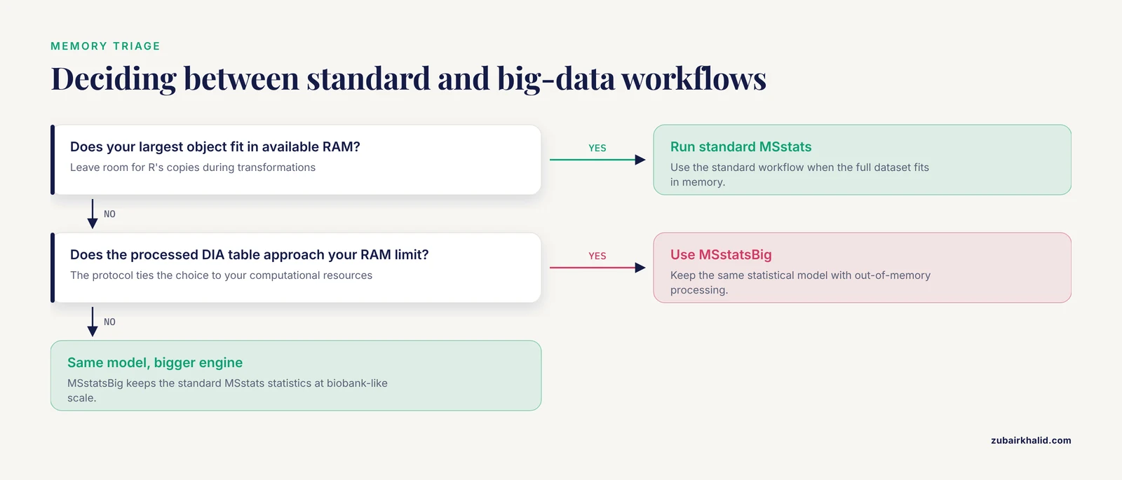
You have a next-generation DIA experiment processed with FragPipe, and the MSstats input table exceeds your workstation's RAM. The updated MSstats protocol describes exactly this decision point. For datasets that fit, run standard MSstats workflows. For datasets too large for standard memory, use the MSstatsBig companion package, which was built to keep the same statistical analysis available at biobank-like scale [3]. The decision rule from the protocol is explicit. The choice of workflow depends on the user's computational resources [3]. Concretely, measure the size of your FragPipe output, compare it against your available RAM, and pick the companion package when the ratio approaches one.
Scenario 2. Whole-genome bisulfite sequencing at cohort scale
Each sample carries more than 100 GB of raw data, and you have a cohort. The scmeth-based pipelines take raw data to CpG-level methylation estimates and run with identical results on a single computer, an HPC cluster, or Google Cloud Compute resources, which solves two problems at once. You get scalability to whole-genome and single-cell scale, and you get comparability with public data because everything passes through the same pipeline [1]. The lesson for any package comparison is that identical results across compute environments is a feature worth paying for, because it converts infrastructure changes from a scientific risk into an administrative task.
Scenario 3. Genomic prediction with Bayesian marker effects on a large pedigree
You need to compare BayesB, BayesC, and BayesR marker effect estimates on tens of thousands of markers across multivariate, repeated observations with missingness. R implementations exist for each algorithm individually, but fitting them across separate software would confound algorithm differences with implementation differences. BESSiE exists precisely because script based environments like R may not handle large-scale marker data or exploit model properties that save time and RAM, and because it implements GBLUP, SNP-BLUP, BayesA, BayesB, BayesC, and BayesR in one command-line program where switching algorithms requires small parameter file changes [2]. The correct architecture here is a shell or R script that writes the parameter files, calls the BESSiE executable, and parses results back into R for plotting and validation.
Scenario 4. Polygenic risk scores on a biobank cohort
You have imputed genotype data for hundreds of thousands of individuals and need PRS across many target traits and P value thresholds. PRSice-2 was built for biobank-scale data, handles both genotyped and imputed input, supports multiple inheritance models and multiple traits simultaneously, and was benchmarked as dramatically faster and more memory-efficient than PRSice-1, LDpred, and lassosum with comparable predictive power [6]. Here the comparison between r package large genomic data comparison options resolves quickly, because the benchmark evidence at the correct scale is direct [6]. Your R script's job is to prepare phenotype and covariate files, call the tool, and visualize results.
Scenario 5. Choosing a batch effect correction method
Your longitudinal metabolomics study shows overtime signal drift, and you cannot decide between correction methods. Rather than eyeballing PCA plots after each candidate method, DBnorm inspects the dataset structure at both the batch scale and the individual metabolic feature scale, assigns a score for model performance on data correction, and helps identify the best fitting model per dataset, demonstrated on two large-scale metabolomics datasets [8]. This pattern, using a dedicated R package to run the comparison itself, also appears in CNV calling [5] and in multi-omics factor analysis, where a published R package implements the cross-validation framework so others can evaluate additional methods and datasets [15]. When several packages could each do your analysis, the highest-leverage package to adopt is sometimes the one that compares them.
Common Mistakes and Limitations
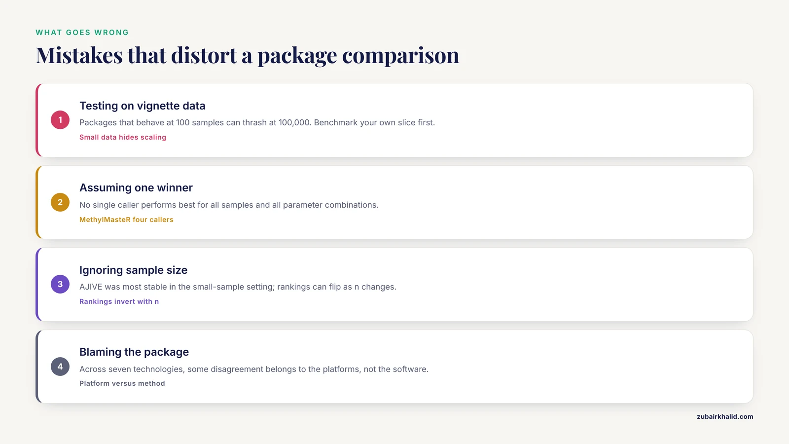
Testing scale behavior on the package's example data. Vignette datasets are small by design. Packages that behave gracefully at 100 samples can fragment memory or thrash at 100,000. The DIA proteomics field rewrote its statistical tooling because tools originally designed with smaller datasets in mind struggled with next-generation experiment scale [3]. Reproduce that lesson deliberately by benchmarking on a slice of your own data before committing.
Assuming one winner exists. The MethylMasteR comparison of four methylation CNV callers found that because the calling algorithms themselves differ, no single software performs best for all samples and all parameter combinations [5]. The same caution applies to any package comparison. Package pros and cons are conditional on your data type, sample size, and parameters, not absolute.
Ignoring sample size interactions. Method comparisons can invert as n changes. In the multi-omics evaluation, all compared methods showed consistency and no overfitting in the large-sample setting, but AJIVE was the most stable in the small-sample setting [15]. A package chosen on the basis of a large-cohort benchmark may be the wrong choice for your 30-patient study.
Confusing platform differences with method differences. When classifiers or measurements move across platforms, agreement changes for reasons unrelated to software quality. Two Burkitt versus diffuse large B cell lymphoma classifiers built on different Affymetrix platforms and fresh-frozen tissue had to be carefully assessed for transferability before a new classifier was built for Illumina DASL data from paraffin-embedded samples [17]. And across seven genomic measurement technologies, consensus modeling identified technology-specific and locus-specific tendencies without any gold standard to arbitrate [16]. If your package comparison spans platforms, some of the measured disagreement belongs to the platforms.
Treating computation time as irrelevant. Simulation work on global tests for functional gene sets found that three approaches had comparable power in many settings while computation times differed considerably [14]. When a genome-wide analysis multiplies any per-unit cost by millions of units, the slower statistically equivalent method is the wrong choice.
Skipping QC as a first-class step. GWAtoolbox exists because QC of large numbers of GWAS result files, checking formatting, quality, and cross-study consistency, needs to run in minutes rather than days, with plots that expose systematic bias between studies [7]. Whichever analysis package you choose, budget for a QC layer, and prefer packages that integrate with one.
Confusing a package with its scope. LocusPackRat prioritizes candidate genes in broad GWAS loci [11]. AlignStatPlot analyzes and visualizes existing alignments [12]. GenomeTornadoPlot visualizes CNVs, it does not call them [9]. PhyloCorrelate infers gene-gene functional associations from phylogenetic profiles [13]. Reading the abstract-level claims carefully prevents the most frustrating failure mode, discovering after a week of work that the package addresses an adjacent problem.
One general limitation applies to everything above. Package benchmarks, caller comparisons, and method rankings are evidence about populations of datasets, and any individual project can behave atypically, so the final validation is always a pilot run on your own data, reviewed with collaborators who know the biology and the statistics involved.
Frequently Asked Questions
Do I need Bioconductor to work with large genomic data in R?
No, but it is usually the right starting point. Bioconductor's shared data containers let QC, analysis, and visualization packages exchange data without conversion code, which matters at scale, and several large-scale packages such as scmeth are built on it [1]. You will likely still call standalone engines for the heaviest computations.
How large does my dataset need to be before memory becomes the deciding factor?
There is no fixed threshold, but the deciding comparison is your largest object size against available RAM, with room for R's copies during transformations. Whole-genome bisulfite sequencing exceeding 100 GB of raw data per sample is firmly beyond in-memory territory [1], and DIA proteomics experiments that will not load into a standard computer's memory call for a companion big-data package [3]. If you are unsure, benchmark a subset and extrapolate.
Should I use a standalone tool instead of an R package for very large analyses?
Use a standalone engine when computation or memory is the bottleneck and an R package when integration and statistics are. BESSiE was created because R may not handle large-scale genomic marker data or exploit model-level savings in time and RAM [2], and PRSice-2 was benchmarked as faster and more memory-efficient than alternative PRS software at biobank scale [6]. Orchestrate such tools from R scripts so your workflow stays in one place.
How do I compare two R packages fairly on my own data?
Run both on the same representative slice, with the same input format, the same parameters where they translate, and the same hardware, and record runtime, peak memory, and agreement of results. Dedicated comparison frameworks show how rigorous this can be, from DBnorm scoring batch correction models on large datasets [8] to MethylMasteR comparing four CNV callers inside a standardized Docker container [5]. Publish your comparison script alongside your analysis.
What is MSstatsBig and when do I need it?
MSstatsBig is a companion R package to MSstats, built for DIA mass spectrometry datasets too large to fit into a standard computer's memory, and the FragPipe-based protocol demonstrates it as the workflow choice when computational resources cannot hold the full dataset [3]. You need it when your processed DIA table approaches your RAM limit and you want to keep the standard MSstats statistical model rather than switching methods.
How do I keep a large R genomic analysis reproducible?
Pin versions, containerize, and route all samples through one pipeline. Deploying an R package comparison as a Docker image standardized the MethylMasteR framework across environments [5], and the scmeth pipelines produce identical results on a single computer, an HPC cluster, or cloud resources specifically to ensure reproducibility and comparability with public data [1]. Record package versions at run time and store them with your results.
Sources
- A (fire)cloud-based DNA methylation data preprocessing and quality control platform.
- BESSiE: a software for linear model BLUP and Bayesian MCMC analysis of large-scale genomic data.
- An MSstats workflow for detecting differentially abundant proteins in large-scale data-independent acquisition mass spectrometry experiments with FragPipe processing.
- Bayesian hybrid index and genomic cline estimation with the R package gghybrid.
- MethylMasteR: A Comparison and Customization of Methylation-Based Copy Number Variation Calling Software in Cancers Harboring Large Scale Chromosomal Deletions.
- PRSice-2: Polygenic Risk Score software for biobank-scale data.
- GWAtoolbox: an R package for fast quality control and handling of genome-wide association studies meta-analysis data.
- DBnorm as an R package for the comparison and selection of appropriate statistical methods for batch effect correction in metabolomic studies.
- GenomeTornadoPlot: a novel R package for CNV visualization and focality analysis.
- PyComplexHeatmap: a Python package to visualize multimodal genomics data.
- LocusPackRat: an R package to support prioritizing candidate genes from large GWAS intervals with standardized evidence aggregation.
- AlignStatPlot: An R package and online tool for robust sequence alignment statistics and innovative visualization of big data.
- PhyloCorrelate: inferring bacterial gene-gene functional associations through large-scale phylogenetic profiling.
- Comparison of global tests for functional gene sets in two-group designs and selection of potentially effect-causing genes.
- Consistency and overfitting of multi-omics methods on experimental data.
- Evaluation of cross-platform and interlaboratory concordance via consensus modelling of genomic measurements.
- Transferring genomics to the clinic: distinguishing Burkitt and diffuse large B cell lymphomas.