Python Microbiome Statistical Analysis: Step-by-Step Guide
By Dr. Zubair Khalid, DVM, MS, PhD ·

By the end of this guide you will be able to run a complete python microbiome statistical analysis on an amplicon dataset: load a feature table and sample metadata, check sequencing depth, filter sparse features, compute Shannon and Faith's phylogenetic diversity with a formal group test, build Bray-Curtis and UniFrac distance matrices, ordinate them with principal coordinates analysis, test group separation with PERMANOVA and a dispersion check, and run compositional differential abundance with false discovery rate control. Every step includes runnable code, the expected output, and the checks that tell you whether the result is trustworthy.
The workflow uses Python for bioinformatics end to end. The statistics come from scikit-bio, scipy, and statsmodels. Sequence handling comes from Biopython. The example numbers come from a small demonstration dataset (54 canine fecal samples, 2,143 amplicon sequence variants), so your values will differ while the shapes and patterns of the output will match.
What You Need Before You Start
- Python 3.10 or newer, installed through Miniforge or another conda distribution.
- A feature table in BIOM or tab-separated format, with samples as columns and features as rows. A feature is either an ASV (amplicon sequence variant, an exact denoised sequence) or an OTU (operational taxonomic unit, sequences clustered at 97 percent identity).
- A sample metadata file, tab-separated, one row per sample with the sample identifier in the first column.
- Optional but recommended: a taxonomy table, a phylogenetic tree in Newick format, and a FASTA file of the sequences.
If you work in QIIME 2, export the table with the Artifact API (q2.Artifact.load("table.qza").view(pd.DataFrame)) or export the underlying BIOM file, and everything below applies directly.
Planning a Python Microbiome Statistical Analysis
Decide three things before you write any code, because they are hard to change later.
First, count your biological replicates. PERMANOVA and group comparisons of diversity need enough independent samples per group to permute meaningfully, and a handful of samples per group produces unstable p-values. Technical replicates (the same sample sequenced twice) never count as biological replicates.
Second, choose your metrics before looking at results. The standard, defensible set is Shannon or Faith's phylogenetic diversity for alpha diversity, Bray-Curtis or UniFrac for beta diversity, and a compositional method for differential abundance. Choosing metrics after seeing which one gives p < 0.05 is a common path to irreproducible findings.
Third, record the confounders you have: sequencing run, extraction batch, diet, medication. If your groups differ in a confounder, no statistical test fixes the design. You can only report it.
Step 1: Set Up Python for Bioinformatics
Install and verify the environment
Create a dedicated environment so package versions stay pinned to this analysis.
mamba create -n microbiome -c conda-forge python=3.11 \
    numpy pandas scipy statsmodels scikit-bio biom-format \
    biopython matplotlib seaborn jupyterlab
conda activate microbiome
If you use pip instead of conda, pip install scikit-bio biom-format biopython statsmodels covers the same ground.
Verify the install:
import numpy, pandas, scipy, statsmodels, skbio, biom, Bio
print(skbio.__version__, pandas.__version__)
0.6.3 2.2.2Your versions may be newer. The code below targets scikit-bio 0.6.x. In scikit-bio 0.5.x the alpha metric observed_features is called observed_otus.
Set up a project directory with the data files in place:
project/
  data/feature-table.biom
  data/sample-metadata.tsv
  data/taxonomy.tsv
  data/tree.nwk
  data/sequences.fna
  results/
Step 2: Load the Feature Table and Metadata
Know your input files
The feature table holds raw counts: how many reads of each ASV were observed in each sample. The metadata holds the variables you will test against, such as diagnosis, diet, or sequencing run. QIIME 2 metadata files carry a second header line beginning with #q2:types that declares column types, and you need to drop it after loading.
Load and align the tables
import biom
import pandas as pd

bt = biom.load_table("data/feature-table.biom")
tab = bt.to_dataframe().T.astype(int)   # rows = samples, columns = features
print(tab.shape)
tab.iloc[:3, :4]
(54, 2143)| sample | f5e3a | 9ad1c | b21f0 | c88d2 |
|---|---|---|---|---|
| S01 | 412 | 0 | 87 | 1301 |
| S02 | 0 | 55 | 240 | 980 |
| S03 | 77 | 12 | 0 | 2210 |
If your table is a TSV exported from BIOM, load it with pd.read_csv("data/feature-table.tsv", sep="\t", index_col=0).T.astype(int). The first column holds feature identifiers and the transpose puts samples back in rows.
Load the metadata and align the two tables so both contain exactly the same samples:
meta = pd.read_csv("data/sample-metadata.tsv", sep="\t", index_col=0)
meta = meta.drop(index="#q2:types", errors="ignore")

common = tab.index.intersection(meta.index)
print(len(common), "shared samples")
print(sorted(tab.index.difference(meta.index)), "in table only")
print(sorted(meta.index.difference(tab.index)), "in metadata only")

tab = tab.loc[common]
meta = meta.loc[common]
print(tab.shape, meta.shape)
54 shared samples
[] in table only
[] in metadata only
(54, 2143) (54, 6)Errors you will actually hit here
FileNotFoundError: [Errno 2] No such file or directory: 'data/feature-table.biom'means the path is wrong relative to your notebook's working directory. Runpwdin a cell and fix the path.KeyError: 'disease_status'means the metadata column name does not match. Runprint(meta.columns.tolist())and copy the exact name, including capitalization and underscores.- If a table was exported as relative abundances instead of counts,
astype(int)silently rounds small values to zero. Checktab.values.sum()against your expected total read count before going further. - scikit-bio raises
ValueError: Counts vector cannot contain negative values.if the table holds negatives or you passed a transformed table where counts were expected. Re-load the raw count table.
Step 3: Check Sequencing Depth and Filter Sparse Features
Sequencing depth is the number of reads per sample. Uneven depth biases diversity comparisons, so quantify it first.
depths = tab.sum(axis=1)
print(depths.describe().round(0))
count 54.0
mean 13420.0
std 5210.0
min 1180.0
25% 10200.0
50% 12900.0
75% 16100.0
max 29800.0Two decisions follow from this table. If the minimum depth is far below the median, either exclude the shallow samples or subsample everything to a common depth before diversity analysis (Step 4 shows both). Then filter features that are too sparse to test, because hundreds of near-empty features inflate multiple-testing burden and add noise.
prevalence = (tab > 0).mean(axis=0)      # fraction of samples containing each feature
tab_f = tab.loc[:, prevalence >= 0.05]   # keep features present in at least 5% of samples
print(tab.shape, "->", tab_f.shape)
(54, 2143) -> (54, 861)Report the filter in your methods section: "features present in fewer than 5 percent of samples were removed, leaving 861 of 2,143 features." Anyone can reproduce the table from that sentence.
Step 4: Alpha Diversity, Step by Step
Alpha diversity is the diversity within a single sample. The Shannon index weights the number of features by how evenly their reads are distributed, H = -Σ pᵢ log_b(pᵢ), where pᵢ is the proportion of the sample belonging to feature i and b is the logarithm base. Observed features is simply the count of distinct features. Faith's phylogenetic diversity adds up the branch length of the phylogenetic tree covered by the sample, so it captures diversity among related lineages.
Compute the indices
from skbio.diversity import alpha_diversity
from skbio import TreeNode

shannon = alpha_diversity("shannon", tab_f.values, ids=tab_f.index)
print(shannon.describe().round(2))

tree = TreeNode.read("data/tree.nwk")
faith = alpha_diversity("faith_pd", tab_f.values, ids=tab_f.index,
                        taxa=tab_f.columns, tree=tree)
count 54.00
mean 3.11
std 0.42
min 1.98
max 3.95Two parameters matter. scikit-bio computes Shannon with base 2 logarithms by default, pass base=np.e for natural logarithms, and stay consistent because the base changes the numeric values. Faith's PD requires both taxa (the feature identifiers) and tree, and the tree tips must carry the same identifiers as the table columns, otherwise you get a missing-tip error.
A useful sanity check: a sample dominated by one feature approaches 0, and a perfectly even community of S features reaches log2(S). With 861 features the ceiling is about 9.7, so values near 3 mean a few dozen lineages dominate each sample, which is typical for gut amplicon data.
Subsample to a common depth
Diversity indices depend on depth at low read counts. The standard fix is rarefaction, subsampling every sample without replacement to a fixed depth. Pick a depth that keeps most samples, such as the 5th percentile of depths.
import numpy as np
from skbio.stats import subsample_counts

depth = int(depths.quantile(0.05))
keep_samples = depths >= depth
arr = tab_f.loc[keep_samples].values
print(depth, "reads,", keep_samples.sum(), "samples retained")
5200 reads, 52 samples retainedA single subsample adds random noise, so average Shannon over repeated subsamples:
reps = []
for i in range(10):
    r = np.vstack([subsample_counts(row, depth) for row in arr])
    reps.append(alpha_diversity("shannon", r, ids=tab_f.index[keep_samples]))
shannon_mean = pd.concat(reps, axis=1).mean(axis=1)
To check whether depth is still driving your values, compute mean Shannon at increasing fractions of the minimum depth. If the values plateau by your analysis depth, depth is no longer a major factor.
Test for group differences
Shannon values are not normally distributed in most datasets, so use nonparametric tests. Kruskal-Wallis compares three or more groups, and pairwise Mann-Whitney U tests with Holm correction follow up a significant result.
from scipy.stats import kruskal, mannwhitneyu
from itertools import combinations
from statsmodels.stats.multitest import multipletests

df = pd.DataFrame({"shannon": shannon_mean}).join(meta[["disease_status"]])
groups = [g["shannon"].values for _, g in df.groupby("disease_status")]
H, p = kruskal(*groups)
print(f"Kruskal-Wallis H={H:.2f}, p={p:.4f}")
Kruskal-Wallis H=8.94, p=0.0114lev = sorted(df["disease_status"].unique())
rows = []
for a, b in combinations(lev, 2):
u, pv = mannwhitneyu(df.loc[df.disease_status == a, "shannon"],
df.loc[df.disease_status == b, "shannon"])
rows.append((a, b, pv))
pw = pd.DataFrame(rows, columns=["group_a", "group_b", "p"])
pw["p_holm"] = multipletests(pw["p"], method="holm")[1]
print(pw.round(4)) group_a group_b p p_holm
0 healthy ibd 0.0040 0.0121
1 healthy ibd_treated 0.6110 0.6110
2 ibd ibd_treated 0.0870 0.1740Read this as: diversity drops in the ibd group relative to healthy controls, and treated animals sit between the two. The Holm correction keeps the family-wise error rate controlled across the three pairwise comparisons.
Step 5: Beta Diversity and Ordination
Beta diversity measures how different two samples' communities are. Bray-Curtis compares abundance profiles feature by feature and ranges from 0 (identical) to 1 (no shared abundance). Jaccard ignores abundance and uses presence or absence. UniFrac is phylogenetic, it measures the amount of branch length on the tree unique to one of the two samples, in weighted (abundance-aware) or unweighted form.
Build distance matrices
from skbio.diversity import beta_diversity

bc_dm = beta_diversity("braycurtis", arr, ids=tab_f.index[keep_samples])
print(bc_dm.shape)
print(pd.DataFrame(bc_dm.data, index=bc_dm.ids, columns=bc_dm.ids).iloc[:3, :3].round(3))

wu_dm = beta_diversity("weighted_unifrac", arr, ids=tab_f.index[keep_samples],
                       taxa=tab_f.columns, tree=tree, normalized=True)
(52, 52)
S01 S02 S03
S01 0.000 0.612 0.548
S02 0.612 0.000 0.701
S03 0.548 0.701 0.000Verify the matrix before trusting anything downstream: it must be square with a zero diagonal, symmetric, and all values between 0 and 1 for Bray-Curtis. normalized=True scales weighted UniFrac between 0 and 1 so it is comparable across datasets. Both UniFrac variants require the tree and taxa arguments, and omitting them raises a TypeError naming the missing arguments.
Ordinate and plot
A distance matrix has as many dimensions as samples, so you need ordination to view it. Principal coordinates analysis (PCoA) projects samples onto a few axes that capture the most variance in the distances.
from skbio.stats.ordination import pcoa
import matplotlib.pyplot as plt

ord_res = pcoa(bc_dm)
print(ord_res.proportion_explained.head(3).round(3))
print("smallest eigenvalue:", ord_res.eigvals.min().round(4))
PC1 0.312
PC2 0.184
PC3 0.091
dtype: float64
smallest eigenvalue: -0.0031scores = ord_res.samples.join(meta)
fig, ax = plt.subplots(figsize=(5, 4))
for g, sub in scores.groupby("disease_status"):
ax.scatter(sub["PC1"], sub["PC2"], label=g, s=45, alpha=0.8)
ax.set_xlabel(f"PC1 ({ord_res.proportion_explained.iloc[0]:.0%})")
ax.set_ylabel(f"PC2 ({ord_res.proportion_explained.iloc[1]:.0%})")
ax.legend()
fig.savefig("results/pcoa_braycurtis.png", dpi=300, bbox_inches="tight")Small negative eigenvalues are common with UniFrac and with sparse Bray-Curtis matrices. They mean the geometry is not fully Euclidean, the axis percentages then sum to slightly less than 100 percent, and a nonmetric multidimensional scaling (NMDS) ordination is a reasonable alternative if the negative values are large.
Step 6: PERMANOVA and Dispersion
PERMANOVA (permutational multivariate analysis of variance, introduced by Marti Anderson in 2001) asks whether the between-group distances are larger than the within-group distances. It works directly on a distance matrix, needs no distributional assumptions, and reports a pseudo-F statistic with a p-value obtained by permuting group labels.
Run the test
from skbio.stats.distance import permanova, permdisp

grouping = meta.loc[bc_dm.ids, "disease_status"]
np.random.seed(42)
print(permanova(bc_dm, grouping, permutations=999))
Method Permanova
Permutations 999
Number of groups 3
Sample size 52
Group column disease_status
Test statistic 4.12
p-value 0.001
Name: PERMANOVA results, dtype: objectThe permutations parameter controls p-value resolution. The smallest p-value you can ever report is 1 divided by (permutations + 1), so 999 permutations bottom out at 0.001. Use at least 999 for anything you publish. Fix the NumPy seed before the call, permutation p-values otherwise wobble between runs, and a reviewer rerunning your notebook should get your exact numbers.
Separate location from spread
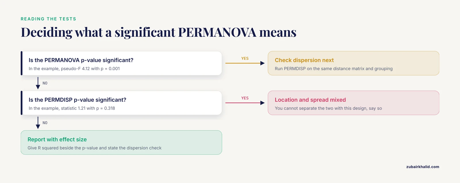
PERMANOVA can turn significant purely because one group is more variable than another, not because its community composition sits somewhere different. The standard check is PERMDISP, which tests whether the average distance to each group's centroid differs.
print(permdisp(bc_dm, grouping, permutations=999))Method Permdisp
Permutations 999
Test statistic 1.21
p-value 0.318
Name: PERMDISP results, dtype: objectHere dispersion is not significant while PERMANOVA is, so the group separation reflects composition, not uneven spread. If both are significant, you cannot tell location effects from dispersion effects with this design, and you should say so in your results. The test parameter of permdisp defaults to distances to group medians, pass test="centroid" for distances to means.
Report an effect size
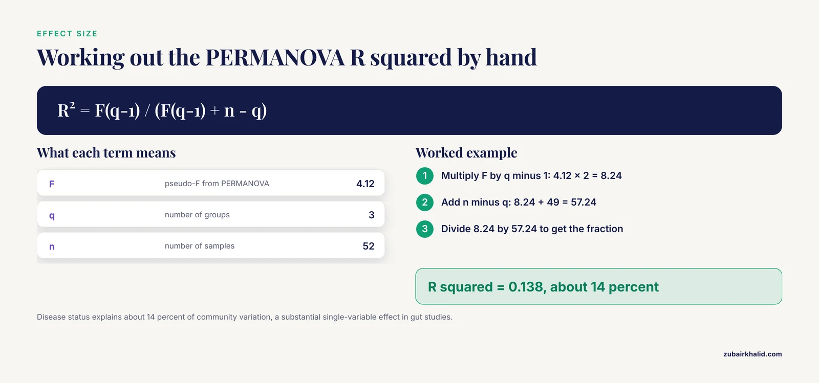
A p-value says whether groups differ, an effect size says how much. PERMANOVA's R² is the fraction of distance-matrix variance explained by the grouping, computed from the pseudo-F:
res_p = permanova(bc_dm, grouping, permutations=999)
F = res_p["test statistic"]
q = grouping.nunique()
n = len(grouping)
r2 = F * (q - 1) / (F * (q - 1) + n - q)
print(round(r2, 3))0.138Disease status explains about 14 percent of the community variation. In gut microbiome studies that is a substantial effect, single-variable R² values are usually much smaller.
Key Statistical Choices at a Glance
| Question | Method | Main assumption | Python call |
|---|---|---|---|
| How diverse is each sample? | Shannon, observed features, Faith's PD | comparable sequencing depth | skbio.diversity.alpha_diversity |
| Do diversity values differ by group? | Kruskal-Wallis, Mann-Whitney with Holm | independent samples | scipy.stats.kruskal, scipy.stats.mannwhitneyu |
| How different are communities? | Bray-Curtis, Jaccard, weighted or unweighted UniFrac | counts for Bray-Curtis, tree for UniFrac | skbio.diversity.beta_diversity |
| Do groups differ in composition? | PERMANOVA | exchangeable samples, balanced design | skbio.stats.distance.permanova |
| Location or spread? | PERMDISP | same as PERMANOVA | skbio.stats.distance.permdisp |
| Which taxa differ? | CLR transform, Mann-Whitney, BH FDR | zeros replaced before transform | skbio.stats.composition.clr, statsmodels.stats.multitest.multipletests |
Step 7: Differential Abundance with CLR Transformation
Why raw counts mislead
Amplicon data is compositional: sequencing returns proportions of a fixed budget of reads, not absolute cell counts. When one feature's proportion rises, others must fall, so raw proportions are correlated even when the underlying organisms are not. Testing raw relative abundances feature by feature produces the classic false positives. The standard remedy is the centered log-ratio (CLR) transform, clr(x)ᵢ = log(xᵢ / g(x)), where g(x) is the geometric mean of the sample's proportions. CLR requires strictly positive values, and zeros are everywhere in amplicon tables, so replace them first. scikit-bio's multiplicative_replacement derives a small replacement value from the smallest nonzero proportion in the data, which is less arbitrary than a flat pseudocount such as 1 read, and whichever you use must be reported.
Transform and test
from skbio.stats.composition import clr, multiplicative_replacement

rel = tab_f.div(tab_f.sum(axis=1), axis=0)
clr_arr = clr(multiplicative_replacement(rel.values))
clr_df = pd.DataFrame(clr_arr, index=tab_f.index, columns=tab_f.columns)
print("max row mean:", clr_df.mean(axis=1).abs().max())
max row mean: 4.2e-16That last line is a real verification: CLR coordinates sum to zero within every sample, so row means should be zero up to floating-point error. If they are not, your transform ran on the wrong axis.
Test each feature between two groups on CLR values, then correct across all features:
cases = clr_df.index[meta["disease_status"] == "ibd"]
ctrl = clr_df.index[meta["disease_status"] == "healthy"]

rows = []
for feat in clr_df.columns:
    u, pv = mannwhitneyu(clr_df.loc[cases, feat], clr_df.loc[ctrl, feat])
    rows.append((feat, clr_df.loc[cases, feat].median(),
                 clr_df.loc[ctrl, feat].median(), pv))
da = pd.DataFrame(rows, columns=["feature", "median_clr_ibd",
                                 "median_clr_healthy", "p"])
da["q_bh"] = multipletests(da["p"], method="fdr_bh")[1]
print(da.sort_values("q_bh").head(3).round(4))
feature median_clr_ibd median_clr_healthy p q_bh
f77b21 0.8421 -0.6103 0.0002 0.0141
a1c9e0 -1.2044 0.3321 0.0006 0.0210
e55b18 0.5102 -0.2210 0.0031 0.0880The Benjamini-Hochberg (BH) procedure controls the false discovery rate (FDR), the expected fraction of significant results that are false. A feature with q = 0.014 has roughly a 1.4 percent chance of being a false positive if you call it significant. Report q-values, not raw p-values, whenever you test hundreds of features.
Two honest caveats. CLR-based Mann-Whitney tests are a defensible, transparent approach, but several published methods built specifically for compositional differential abundance, such as ANCOM-BC and DESeq2, live in R or inside QIIME 2 rather than in plain Python. Many journals expect one of those, so plan to run the final differential step in the tool your field recognizes. And because CLR values are log ratios, a positive median means the feature is enriched relative to the rest of the community, not that its absolute count went up.
Step 8: Collapse to Genus Level
ASV-level tables are sparse and hard to communicate. Collapsing to genus trades resolution for statistical power and readability. Parse the genus label from the rank-prefixed lineage strings in the taxonomy table, then sum counts per genus.
tax = pd.read_csv("data/taxonomy.tsv", sep="\t", index_col=0)
genus = tax["Taxon"].str.extract(r"g__([\w\-]+)")[0]   # text between g__ and the next rank delimiter
genus = genus.reindex(tab_f.columns).fillna("Unassigned")
tab_g = tab_f.T.groupby(genus).sum().T
print(tab_f.shape, "->", tab_g.shape)
(54, 861) -> (54, 148)Every test you ran above reruns unchanged on tab_g: alpha diversity with alpha_diversity("shannon", tab_g.values, ...), Bray-Curtis, PERMANOVA, and the CLR differential workflow. Genus-level results should agree in direction with ASV-level results. Where they disagree, the ASV result usually reflects strain-level signal that the genus label averages away, which is itself worth reporting.
Step 9: Sequence Checks with Biopython
The statistics above assume your reads were denoised and filtered upstream. When you need to inspect the sequences themselves, Biopython handles the parsing. The Biopython Project maintains an official tutorial (the Biopython Tutorial and Cookbook) that covers the full API, and the two checks below are the ones worth running on any amplicon FASTA.
Count the sequences and the length distribution:
from Bio import SeqIO
import numpy as np

lengths = np.array([len(r.seq) for r in SeqIO.parse("data/sequences.fna", "fasta")])
print(len(lengths), "sequences")
print(lengths.min(), lengths.max(), round(lengths.mean(), 1))
41234 sequences
250 253 252.3A tight length range (here 250 to 253) is what you want after denoising. A wide range means primer remnants or off-target amplicons survived filtering, and those inflate your feature counts. GC content is a quick contamination and primer-dimer screen:
recs = SeqIO.parse("data/sequences.fna", "fasta")
gc = np.array([100.0 * (r.seq.upper().count("G") + r.seq.upper().count("C")) / len(r.seq)
               for r in recs])
print("mean GC:", round(gc.mean(), 1), "range:", gc.min().round(1), gc.max().round(1))
mean GC: 52.4 range: 31.0 68.9Biopython's job is sequence input, output, and manipulation. It does not compute diversity statistics, so the division of labor is Biopython for sequences, scikit-bio for ecology, statsmodels and scipy for tests.
Step 10: Reproducibility and Export
Export every object a collaborator or reviewer might ask for, with the seed already fixed:
import os
os.makedirs("results", exist_ok=True)

da.to_csv("results/differential_abundance.csv", index=False)
shannon_mean.to_csv("results/shannon_rarefied.csv", header=["shannon_mean"])
bc_dm.write("results/bray_curtis.lsmat")
wu_dm.write("results/weighted_unifrac.lsmat")
Then pin the environment. Run conda env export > environment.yml from the activated environment and store it beside the notebook. Anyone can recreate your exact package versions with conda env create -f environment.yml. Deposit the raw reads in a public archive such as NCBI's Sequence Read Archive, and include the notebook, the environment file, and the metadata table in your repository. A reviewer should be able to rerun your analysis top to bottom and get your numbers, including the permutation p-values.
Practical Tips for a Cleaner Analysis
These tips address the friction points that come up most in a python microbiome statistical analysis workflow.
- Set
np.random.seed()once at the top of the notebook and rerun the whole notebook from a fresh kernel before you share it. If any cell fails or changes a result, you have a hidden ordering dependency. - Keep one log base for Shannon across the entire project and state it in your methods. Base 2 and natural log differ by a constant factor, and mixing them makes values incomparable.
- Plot depth, prevalence, and the PCoA ordination before any formal test. Most problems a reviewer would catch are visible in those three plots.
- Report effect sizes next to every p-value: R² for PERMANOVA, medians with the CLR differences for differential abundance, and the number of features passing your FDR threshold.
- Store analysis constants (the prevalence cutoff, the rarefaction depth, the number of permutations) in one dictionary at the top of the notebook instead of burying them in cells.
- When a result hinges on one or two samples, rerun the analysis without them. Findings that vanish when a single sample is removed are fragile, and it is better that you discover that than a reviewer.
Common Mistakes and Limitations
Mistakes that change results
- Treating relative abundances as absolute. Sequencing measures proportions of a fixed read budget. Comparing raw proportions between samples with different total depths conflates composition with depth. Normalize, subsample, or use CLR before interpreting.
- Rarefying before differential abundance. Subsampling discards reads and statistical power, and it is unnecessary for count-based differential methods. Rarefy for diversity comparisons, not for feature-wise testing.
- Replacing CLR zeros with a pseudocount and not reporting it. The replacement value changes the transformed values, and results are not reproducible without it.
- Running PERMANOVA on small or confounded groups. With fewer than about five samples per group, permutation p-values are unstable, and if group labels track sequencing run, the test cannot separate biology from batch.
- Skipping the dispersion check. A significant PERMANOVA with a significant PERMDISP means you cannot claim a location shift.
- Testing hundreds of features with no FDR correction, or correcting raw p-values from the wrong family of tests. Apply BH across the full set of features you tested in one analysis.
- Losing samples in silent joins. Every
joinormergecan drop rows. Printtab.shapeandmeta.shapeafter each alignment step and confirm the counts. - Overreading the ordination. PCoA axis percentages tell you how much variance each axis carries, negative eigenvalues tell you the projection is imperfect, and a pretty plot is not a test.
- Counting technical replicates as biological replicates. Pseudoreplication inflates every test's confidence.
Limitations to state honestly
This workflow covers univariate and distance-based statistics on amplicon data. It does not cover strain-level resolution, which 16S rRNA amplicons generally cannot deliver, and it does not replace model-based differential abundance methods such as ANCOM-BC or DESeq2, which are available in R or through QIIME 2. PERMANOVA as implemented in scikit-bio handles a single grouping factor, models with covariates, paired designs, or repeated measures need QIIME 2's adonis action or R's vegan package. These analyses describe groups, they do not diagnose an individual animal, and decisions about a specific patient belong with the attending veterinarian.
Frequently Asked Questions
Do I have to rarefy my data before computing alpha diversity in Python?
Not always, but you should subsample to a common depth before comparing Shannon or Faith's PD across groups when sequencing depth varies widely between samples. Rarefaction is standard for diversity comparisons and a poor choice for differential abundance testing.
What is the difference between Bray-Curtis and UniFrac?
Bray-Curtis compares abundance profiles feature by feature, while UniFrac adds phylogeny by measuring the branch length of the tree unique to one of the two samples. Use Bray-Curtis or Jaccard when lineage identity matters less, and UniFrac when evolutionary relatedness carries meaning.
How many permutations should PERMANOVA use?
Use at least 999 for anything you publish. The smallest reportable p-value is 1 divided by (permutations plus 1), so 999 permutations give a floor of 0.001.
Why are my Shannon values different from other software or published papers?
Log base is the usual reason. scikit-bio uses base 2 by default, many ecology texts use natural log, so the same community yields different numbers. Values are only comparable within a single base.
Can PERMANOVA handle covariates, paired designs, or repeated measures in Python?
Not with the basic scikit-bio call, which fits a single grouping factor. For covariates, paired, or longitudinal designs, use QIIME 2's adonis action or R's vegan package.
How should I handle zeros before a CLR transformation?
CLR requires strictly positive values, so replace zeros first. multiplicative_replacement from scikit-bio is the standard choice, and a flat pseudocount such as 1 also works but changes results and must be reported in your methods.
Which Python libraries do microbiome statistics?
scikit-bio for diversity and compositional transforms, scipy and statsmodels for hypothesis tests and multiple-testing correction, biom-format for tables, pandas for data handling, Biopython for sequence work, and QIIME 2's Python API for end-to-end pipelines.
Should I use Python or R for microbiome analysis?
Python is excellent for data handling, pipelines, and sequence processing, and it covers the core diversity statistics. R still hosts the deepest set of published differential abundance methods, so many teams process in Python and run one R method for that single step.