How to Set Up Python for Bioinformatics
By Dr. Zubair Khalid, DVM, MS, PhD ·

Setting up Python for bioinformatics means installing the Python interpreter inside an isolated, version-controlled environment and then adding the scientific libraries, such as Biopython, NumPy, pandas, and Jupyter, that let you read sequence files, run analyses, and record exactly how each result was produced. A correct setup keeps every project's dependencies separate, so that updating one tool never silently breaks another analysis.
This matters because modern biological analysis is software-dependent from the first FASTQ file to the final figure. Researchers have shown that identical code can produce different results depending on which package versions are installed, and that incomplete documentation of dependencies and versions is a leading reason bioinformatics analyses fail to reproduce [1]. The setup you build in the first hour of a project determines whether your work is reproducible months later, whether a collaborator can run your script, and whether you can rerun an analysis when a reviewer asks a question a year after publication. This guide walks through the full python for bioinformatics setup, from choosing an installation path to writing your first Biopython script, with worked commands you can type as written.
What Is Python for Bioinformatics Setup? A Plain Definition
When people ask what is python for bioinformatics setup, they are usually asking about two different things at once. The first is the mechanical task: putting the Python language and a set of scientific libraries onto a computer in a way that is stable, isolated, and documented. The second is the workflow decision: choosing which tools and which environment model (local environments, containers, or cloud notebooks) fit the kind of biology you do.
To keep the vocabulary straight, four terms get confused constantly:
- Python is the programming language and the interpreter program that runs your code.
- Biopython is a specific library of Python code for biological data, with parsers for FASTA, FASTQ, GenBank, PDB, and other formats, plus tools for sequence manipulation, alignment interfaces, and file conversion.
- conda (and its faster engine mamba) is a package and environment manager. It installs Python itself, libraries with compiled components, and non-Python tools, and it keeps each project in its own isolated environment.
- Jupyter is an interactive notebook interface that mixes code, output, and notes in a single document, which is why it dominates bioinformatics teaching and exploratory analysis.
A python for bioinformatics setup, explained simply, is the combination of these four pieces configured so they cannot interfere with each other. You never install packages directly into the system-wide Python. You create one environment per project, install that project's libraries there, and record the exact versions in a file that anyone can use to rebuild the same setup.
The scale of the Python ecosystem in biology explains why the setup step deserves this care. Published Python-based tools now cover nearly every subfield: PyMACS automates the full GROMACS molecular dynamics pipeline from structure cleanup through trajectory analysis [2]. easyPheno provides a framework for phenotype prediction from genotype data with automated hyperparameter search, installable from the Python Package Index or through Docker [3]. pyCaverDock exposes ligand-transport calculations through a Python 3 application programming interface (API) [4]. EasyFlyTracker analyzes Drosophila locomotor activity from video [5], and BMT bundles DNA analysis, translation, gene prediction, and sequence alignment into a single desktop application built from Python packages [6]. Every one of these projects assumed a working Python environment as its starting point.
Why the Setup Matters More in Biology Than in Most Fields
In web development, a broken dependency usually means a broken website that someone notices immediately. In bioinformatics, a broken or drifted environment can produce numbers that look plausible and are quietly wrong. The FairFlow project describes the core problem precisely: bioinformatics analyses depend on external software that itself relies on further programs, each with its own release cycle, and because tools are updated to fix bugs and add features, the same script can give different results on different machines when dependency versions differ [1].
Three practical consequences follow from this, and they shape every recommendation in this guide.
First, isolation. If you install all packages into one shared location, the versions demanded by one project conflict with another. A genomics pipeline that needs one version of a library and a single-cell analysis that needs another cannot coexist there. Environment managers solve this by giving each project its own directory of packages.
Second, version recording. Writing down the exact versions of Python and every installed package is what turns a working setup into a reproducible one. Version-locked environments and containers are the two established mechanisms for this, and both appear throughout the published bioinformatics literature [1],.
Third, low-friction onboarding. Students and collaborators abandon projects when the setup takes days. Teaching studies have shown that cloud-hosted notebooks, which require no local installation at all, removed technical barriers for biomedical students with varied computing setups and increased their confidence with bioinformatics tools [8]. Containers serve the same goal for deployed analyses. When the CoGAPS team packaged their single-cell NMF workflow, they provided a procedure for running the Python implementation inside Docker precisely so that users would not have to rebuild a complex dependency chain by hand [7].
Choosing Your Setup Path: Four Options Compared
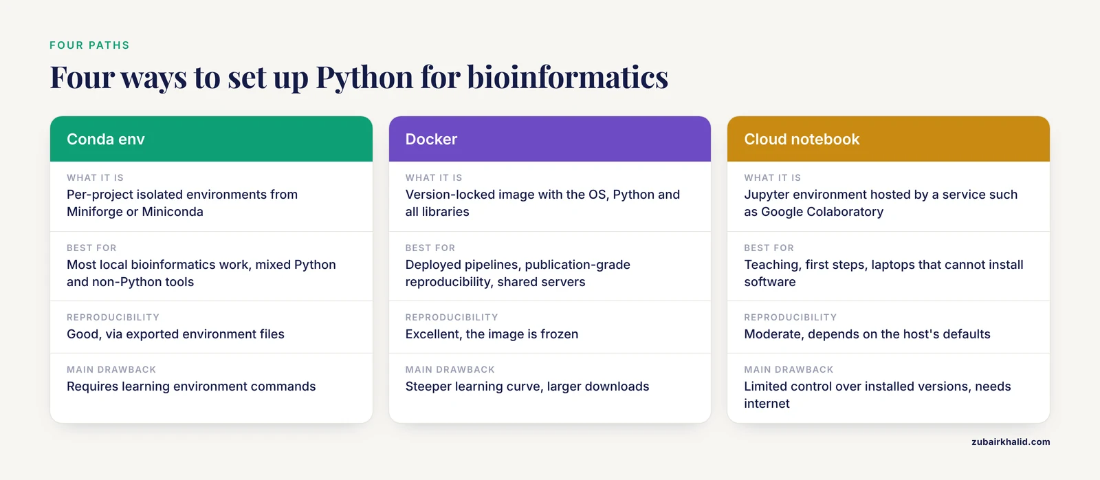
There is no single correct way to set up Python for bioinformatics. The right choice depends on your hardware, your field, and who needs to rerun your work. The table below compares the four paths used in practice.
| Setup path | What it is | Best for | Reproducibility | Main drawback |
|---|---|---|---|---|
| System Python | The interpreter preinstalled on macOS or Linux, with packages added globally | Quick one-off scripts, learning basic syntax | Poor, versions drift and conflict | Breaks operating system tools, no isolation |
| Conda or mamba environment | Per-project isolated environments from Miniforge or Miniconda | Most local bioinformatics work, mixed Python and non-Python tools | Good, via exported environment files | Requires learning environment commands |
| Docker container | A version-locked image containing the OS, Python, and all libraries | Deployed pipelines, publication-grade reproducibility, shared servers | Excellent, the image is frozen | Steeper learning curve, larger downloads |
| Cloud notebook | A Jupyter environment hosted by a service such as Google Colaboratory | Teaching, first steps, laptops that cannot install software | Moderate, depends on the host's defaults | Limited control over installed versions, needs internet |
Most working bioinformaticians combine paths. A conda environment is the daily driver for interactive analysis, a Docker container freezes that environment when results must be published or shared, and cloud notebooks serve students and collaborators who should not have to install anything. Published frameworks illustrate the pattern. easyPheno offers installation both as a standard Python package and through Docker [3], and the CoGAPS protocols include a Docker deployment path alongside a browser-based notebook option for users without programming proficiency [7].
For a first setup, this guide recommends the conda path with Miniforge, because it isolates projects, installs compiled scientific libraries reliably, and exports a record of everything it installed. The steps below assume macOS, Linux, or Windows with the Windows Subsystem for Linux, though the conda commands are identical on all three.
The Step-by-Step Setup
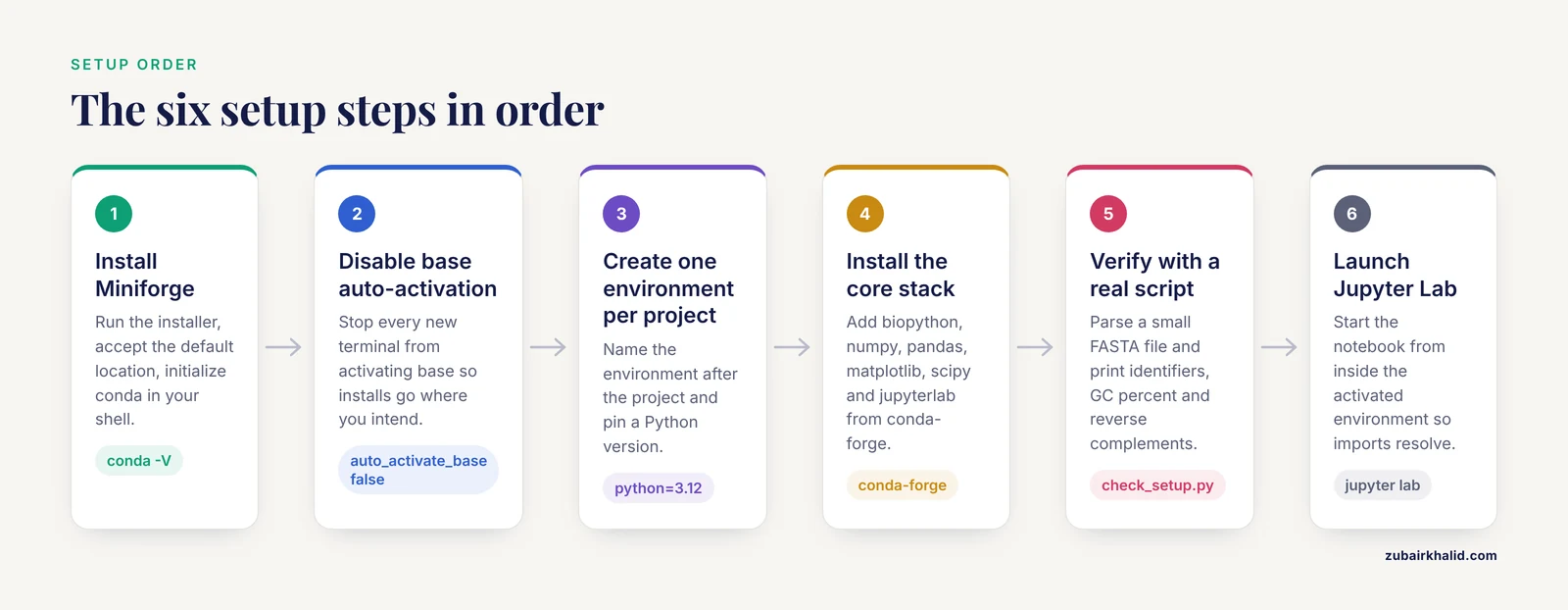
Step 1: Install Miniforge
Miniforge is a minimal distribution of conda built on conda-forge, a community channel that hosts thousands of scientific packages. Download the installer for your operating system from the Miniforge repository on GitHub, then run the installer from a terminal. On a Mac with Apple silicon, the sequence looks like this:
bash Miniforge3-MacOSX-arm64.shAccept the license, accept the default install location, and answer yes when asked whether to initialize conda in your shell. Close and reopen the terminal, then confirm the installation:
conda -VYou should see a version number beginning with a 24 or higher series. If the command is not found, your shell has not loaded the initialization block, which a reopened terminal usually fixes.
Step 2: Stop conda from auto-activating the base environment
By default, every new terminal activates the base environment. Most bioinformaticians turn this off so that scripts run against an explicit environment by choice:
conda config --set auto_activate_base falseThis is a small habit with a large payoff. It prevents the common accident of installing a package into base and later wondering why another project cannot see it.
Step 3: Create one environment per project
Create your first environment, name it after the project, and pin a Python version:
conda create -n rnaseq-intro python=3.12
conda activate rnaseq-intro
The -n flag sets the environment name. After activation, your prompt shows the environment name, and every package you install goes only into that environment. To leave it, type conda deactivate. To see all environments, type conda env list.
Choosing a Python version is a real decision. Python 3.12 is a safe current choice for most scientific libraries in 2026. Some older published tools still require specific older versions, which is exactly why per-project environments exist. When you install a published tool, read its documentation for the supported Python version and build the environment to match.
Step 4: Install the core scientific stack
For a general bioinformatics environment, install the following from the conda-forge channel:
conda install -c conda-forge biopython numpy pandas matplotlib scipy jupyterlabEach package earns its place:
- biopython parses and writes biological file formats and provides sequence objects, translation tables, and interfaces to external tools.
- numpy provides the array data structure that underlies nearly all numerical work.
- pandas provides the DataFrame, the table structure you will use for count matrices, variant tables, and metadata.
- matplotlib produces the standard static plots, and scipy adds statistics and signal processing.
- jupyterlab gives you the notebook interface.
Many fields add specialized packages later. Single-cell work typically adds scanpy and anndata. Structural biology adds MDAnalysis or Bio.PDB. Machine learning adds scikit-learn. The published frameworks described later in this guide show how these stacks grow around a project.
Some bioinformatics tools are not Python packages at all and cannot come from conda-forge. Sequence aligners, genome assemblers, and similar command-line tools are available through the bioconda channel, which is maintained specifically for bioinformatics software:
conda install -c conda-forge -c bioconda samtoolsThis is one of the quiet strengths of the conda path. One command installs a non-Python aligner and its dependencies into the same isolated environment as your Python code.
Step 5: Verify the installation with a real script
Do not trust a setup until it has parsed a real biological file. Create a small FASTA file called test.fasta with this content:
>demo_seqA
ATGGCCTATGCAATGAAAGGC
>demo_seqB
ATGGCCTTCGCAATGAACGGC
Then run this script, saved as check_setup.py:
from Bio import SeqIO

for record in SeqIO.parse("test.fasta", "fasta"):
    seq = record.seq
    gc = (seq.count("G") + seq.count("C")) / len(seq) * 100
    print(record.id, "length:", len(seq), "GC percent:", round(gc, 1))
    print("reverse complement:", seq.reverse_complement())
Run it with:
python check_setup.pyIf you see sequence identifiers, GC percentages, and reverse complements printed without an import error, your interpreter, Biopython, and file parsing all work together. This single test catches most broken setups.
Step 6: Set up Jupyter Lab
Start the notebook server from inside your activated environment:
jupyter labA browser window opens at a local address. Create a new notebook, and in its first cell run:
import Bio
import numpy
import pandas
print(Bio.__version__)
If this prints a Biopython version number, the notebook is using the correct environment. One frequent trap deserves a warning here. If you start Jupyter from outside the environment, the notebook may import a different Python installation and report that Biopython does not exist, even though it is installed. Always activate the environment first, then launch Jupyter from inside it.
A First Biopython Tutorial: From FASTA to Translation
Because Biopython is the library new bioinformaticians reach for first, this section works through a short biopython tutorial that builds directly on the verified setup. The goal is a script that reads a DNA sequence, reports its properties, and translates it into protein, the kind of task BMT packages into a point-and-click tool for DNA and protein analysis [6], but here done in a dozen lines of code you control.
Start with the same FASTA file from the verification step. Extend the script as follows.
Parsing and inspecting records:
from Bio import SeqIO

records = list(SeqIO.parse("test.fasta", "fasta"))
first = records
print("identifier:", first.id)
print("description:", first.description)
print("sequence:", first.seq)
SeqIO.parse is a generator over the records in the file. Wrapping it in list() loads them all, which is fine for small files. first.seq is a Seq object, which behaves like a string but carries biological methods.
Computing composition and GC content:
from Bio.SeqUtils import gc_fraction

print("GC fraction:", gc_fraction(first.seq))
Biopython provides gc_fraction for GC content so you do not have to recount bases by hand in every script.
The central sequence operations:
seq = first.seq
print("complement:", seq.complement())
print("reverse complement:", seq.reverse_complement())
print("transcription (DNA to RNA):", seq.transcribe())
print("translation:", seq.translate())
Translation follows the standard genetic code by default, converting the DNA sequence into an amino acid string. For the demo sequence, translation stops at the first in-frame stop codon unless you adjust options, which is itself a useful lesson: biological sequence objects encode the rules of molecular biology, not just string operations.
Writing output in another format:
SeqIO.write(records, "test.genbank", "genbank")Format conversion, one of the most repetitive chores in bioinformatics, becomes a single line because Biopython knows the structure of both formats.
The pattern generalizes to real data. Replace test.fasta with a downloaded genome or transcript file, and the same SeqIO.parse loop handles it. This is the everyday working style of python for bioinformatics: parse a standard file, operate on sequence objects with biological methods, write results with pandas or matplotlib, and let Biopython handle the format details.
Python for Bioinformatics Setup Examples from Published Tools
Abstract setup advice becomes concrete when you see how published bioinformatics projects expect to be installed. These python for bioinformatics setup examples, all drawn from the peer-reviewed literature, span the major subfields and illustrate the installation patterns you will meet.
easyPheno, phenotype prediction. The easyPheno framework trains and compares phenotype prediction models ranging from genomic selection to deep learning, with automatic Bayesian hyperparameter optimization, and its developers made it available as a standard Python package installable from the Python Package Index and also via Docker [3]. For your own projects, the lesson is that a well-built tool ends up installable at least two ways. A plain pip install easypheno inside an activated conda environment works for interactive use, while the Docker route guarantees the same versions on every machine.
PyCoGAPS, single-cell analysis. The CoGAPS team published four procedures for non-negative matrix factorization of single-cell RNA-sequencing data. Their Python implementation, PyCoGAPS, was written to improve runtime on large datasets, and one published procedure walks through deploying it in Docker, while another offers a browser-based notebook platform for users without Python proficiency [7]. Notice the design philosophy: one algorithm, four access routes, matched to four user skill levels. Your setup should serve the same range, with a local environment for yourself and a container or notebook for others.
pyCaverDock, enzyme tunnel analysis. pyCaverDock wraps the CaverDock ligand-transport tool in a Python 3 API that automates setup steps and supports screening pipelines, with caching and batch calculation support [4]. API-style tools like this are the reason the isolated environment matters: the API depends on a specific underlying CaverDock installation, and only a per-project environment keeps those coupled dependencies consistent.
PyMACS, molecular dynamics. PyMACS automates the complete GROMACS molecular dynamics workflow, from structure cleanup and force-field-compatible topology generation using CHARMM36 force fields through solvation, minimization, equilibration, production, and analysis, accepting PDB, CIF, and mmCIF inputs across proteins, nucleic acids, and protein-ligand complexes [2]. This is the heavy end of the Python bioinformatics stack. A tool this complex pulls in a simulation engine, force-field data, and parameterization software, which makes manual installation error-prone and makes scripted, environment-based installation nearly mandatory.
EasyFlyTracker, behavioral video analysis. EasyFlyTracker tracks single adult Drosophila in video arenas and quantifies locomotor and sleep activity, with a design emphasizing low cost, easy setup and scaling, and compatibility with different recording systems and common video formats [5]. It shows that the same setup discipline, an installable package with declared dependencies, applies outside sequencing entirely.
BMT, a packaged desktop tool. BMT bundles FastqTrimmer, gene prediction, DNA and protein property analysis, six-frame translation, and pairwise and multiple sequence alignment into a standalone desktop application built from state-of-the-art Python packages [6]. It represents the opposite end of the accessibility spectrum: no visible Python at all. Many collaborators will ultimately consume your work through interfaces like this, which is a reason to keep your underlying code importable and modular.
The common thread across all six projects is the same one this guide has been building: every team had to make an installation decision, document it, and make it repeatable for someone else's computer. The published tools that survive are the ones that treated setup as part of the science.
Recording and Rebuilding: The Reproducibility Layer
A working environment on your laptop is not a setup until it can be rebuilt somewhere else. Two file formats accomplish this, and you should export both after any significant change.
Conda environment files. From inside your activated environment, run:
conda env export > environment.ymlThis writes the environment name, the Python version, the channel configuration, and the exact version of every package into a plain text file. Anyone, including you on a new computer, can recreate it with:
conda env create -f environment.yml
conda activate rnaseq-intro
Commit this file to your project's version control repository alongside the code. The environment file is part of the methods section of a computational paper.
Pip requirement files. When collaborators use pip rather than conda, provide:
pip freeze > requirements.txtinstalled later with pip install -r requirements.txt.
Containers. For publication-grade reproducibility, wrap the environment in a Docker image. The FairFlow framework argues that containerization packages software with all its dependencies, removing version drift between machines, while noting that containers alone have demanded technical expertise and lacked a standard operating procedure, which motivated their automated, version-locked approach to generating pipeline interfaces [1]. The CoGAPS team likewise shipped a Docker deployment procedure for their Python single-cell workflow so that users inherit the exact tested stack rather than rebuilding it [7]. A minimal Dockerfile that layers your environment file onto a Python base image is often all that is needed, and many projects publish their images on Docker Hub so that a collaborator runs one pull command and gets your entire computational environment.
A practical habit ties this layer together. At the end of each working session that involved a new install, re-export the environment file. An environment file that is three months out of date is a reproducibility record that lies.
How a Setup Is Tested and Observed in Practice
Professionals verify a python for bioinformatics setup at three levels, and you should adopt all three.
The first level is import verification, which you already performed in Step 5. Every time you add a package, run a one-line import of it in the interpreter before writing any real code. Import errors caught immediately are trivial. Import errors discovered mid-analysis waste an afternoon.
The second level is version introspection. Run conda list inside the environment to print every installed package and its version, and record that output in your project notes. When a result changes between two runs months apart, this list is the first place you look, because version drift between runs is the canonical cause of irreproducibility in bioinformatics pipelines [1].
The third level is a canary analysis. Keep a tiny script, like the FASTA parsing example above, whose correct output you know by heart. Run it whenever you change the environment. If the canary output changes, you have caught the problem before it contaminates real results. Research groups that maintain rigorous pipelines effectively institutionalize this idea, checking that updates to dependencies do not alter published results before adopting them [1].
In teaching settings, the observation of a good setup looks different. Studies of biomedical master's students using cloud-based interactive notebooks found that eliminating installation friction let students focus on the biological analysis itself, and that the notebooks covered everything from data manipulation to multi-omics applications [8]. If you are teaching or onboarding, the cloud notebook path is the observed best practice for the first day, with local environments introduced once the concepts are secure.
Common Mistakes and Limitations
Every experienced bioinformatician has made most of these mistakes. Treat this section as a checklist.
- Installing everything into base or system Python. This is the single most common failure. Packages accumulate, versions conflict, and eventually nothing can be upgraded without breaking something. The fix is discipline: one named environment per project, created on day one.
- Mixing pip and conda carelessly in the same environment. Both package managers can install the same libraries, and alternating between them can produce inconsistent dependency trees. Establish a convention, such as conda for everything available on conda-forge and bioconda, pip only for packages that exist nowhere else, and pip last.
- Launching Jupyter from the wrong place. As described in Step 6, a notebook started outside your environment will import a different Python and report your packages as missing. Activate first, launch second.
- Never recording versions. A script that ran yesterday and fails today is almost always an environment problem, and without
environment.ymlorrequirements.txtthere is nothing to compare against. Export after every meaningful change. - Assuming published tools install cleanly on any Python. Tools built on compiled scientific libraries can pin specific Python versions. Read the tool's installation documentation before creating the environment, not after the first failed install.
- Treating the cloud notebook as a substitute for a real environment in research. Notebooks are excellent for learning and exploration, as the teaching literature confirms [8], but for a multi-week analysis with publication-grade reproducibility you need recorded, version-locked environments or containers [1], [7].
- Confusing setup with the science. A perfect environment produces no results by itself. Budget your setup time honestly, aim for under an hour on a new project, and get to the data.
One limitation of scope belongs on the record. This guide covers the Python software environment. It does not cover high-performance computing job schedulers, cluster module systems, or licensed software, each of which has its own institutional documentation that supersedes general advice.
Quick Review
- A python for bioinformatics setup combines the Python interpreter, an environment manager such as conda, scientific libraries such as Biopython and pandas, and a record of exact versions.
- Never install project packages into base or system Python. Create one isolated, named environment per project.
- Install the core stack from conda-forge, and use the bioconda channel for non-Python tools such as aligners.
- Verify any new setup by parsing a real FASTA file with Biopython and running a known-output canary script.
- Export
environment.ymlandrequirements.txtafter every meaningful change, and commit them with your code. - Use Docker containers when results must be reproduced exactly on other machines, as published frameworks such as FairFlow and PyCoGAPS do [1], [7].
- Use cloud notebooks for teaching and zero-install first steps, and local environments for real projects [8].
Frequently Asked Questions
Do I need an expensive computer to run Python for bioinformatics?
No. The Python interpreter, Biopython, pandas, and Jupyter all run comfortably on an ordinary laptop, and the free cloud notebook route removes even that requirement, since studies of biomedical students used Google Colaboratory notebooks precisely to equalize access across varied computing setups [8]. Large genomics datasets and molecular dynamics simulations eventually need more compute, but you can learn and complete most sequence-level work on modest hardware.
What is Biopython and do I have to use it?
Biopython is a Python library of parsers and tools for biological data, including FASTA, FASTQ, and GenBank formats, sequence objects with biological methods, and file format conversion. You do not have to use it, but it removes enormous amounts of formatting work, and virtually every Python-based bioinformatics resource assumes some familiarity with it. The short tutorial in this article covers the operations most beginners need first.
Should I install packages with pip or conda?
Use conda from conda-forge and bioconda as your default, because it handles compiled scientific libraries and non-Python tools reliably. Use pip for packages that conda does not provide, and install those last inside the environment. The important rule is consistency within each environment, not purity across all of them.
Why does my setup break when I install everything in one place?
Because different projects need different versions of the same libraries, and a single shared installation can hold only one version at a time. Upgrading a package for one project silently changes it for every other project. Isolated environments fix this by giving each project its own package directory, and version recording makes the state of each environment auditable [1].
Do I need to learn Docker right away?
No. Start with conda environments and version files, which cover daily research work. Add Docker when a project must be shared, published, or run identically on multiple machines. Published frameworks reached the same conclusion: containers give the strongest reproducibility, and tools like easyPheno and PyCoGAPS offer Docker as an installation path for exactly that reason [3], [7].
How much Python do I need to know before starting bioinformatics?
You need variables, loops, functions, lists, and dictionaries, roughly the first few lessons of any Python course. Everything more advanced you will learn on real data. Teaching studies that used interactive notebooks covering Python basics alongside practical bioinformatics applications found that students with no computing background gained confidence and engagement with exactly this approach [8]. Start manipulating sequences within your first week rather than finishing an abstract programming course first.
Sources
- FairFlow: A transparency-first framework for verifiable and reproducible bioinformatics.
- PyMACS: A python-based automation suite for GROMACS molecular dynamics setup, simulation, and analysis.
- easyPheno: An easy-to-use and easy-to-extend Python framework for phenotype prediction using Bayesian optimization.
- pyCaverDock: Python implementation of the popular tool for analysis of ligand transport with advanced caching and batch calculation support.
- EasyFlyTracker: A Simple Video Tracking Python Package for Analyzing Adult Drosophila Locomotor and Sleep Activity to Facilitate Revealing the Effect of Psychiatric Drugs.
- BMT: Bioinformatics mini toolbox for comprehensive DNA and protein analysis.
- Inferring cellular and molecular processes in single-cell data with non-negative matrix factorization using Python, R and GenePattern Notebook implementations of CoGAPS.
- Teaching Python with team-based learning: using cloud-based notebooks for interactive coding education.