How to Create a Publication-Ready Phylogenetic Tree in R with ggtree

By Dr. Zubair Khalid, DVM, MS, PhD · 2026-11-11

By the end of this guide you will be able to take a phylogenetic tree file (Newick, NEXUS, or BEAST output), read it into R, add tip labels, branch support values, clade highlights, and external data such as host species or genome statistics, choose an appropriate layout, and export a vector figure that meets journal figure requirements. You will also know the mistakes that most often produce a rejected or misleading tree figure, and how to check your work before submission.

To follow along you need R (any recent version from CRAN), a text editor, and a tree file produced by a phylogenetic inference program such as IQ-TREE, RAxML, MrBayes, or BEAST. If you do not have a tree yet, the worked example below includes a small Newick string you can use as a stand-in. Everything runs in R, so this is a practical exercise in R for bioinformatics rather than a survey of tree-drawing tools.

Why ggtree produces publication-ready trees

ggtree is an R package built on the ggplot2 grammar of graphics, distributed through Bioconductor, the open-source software project for bioinformatics. Its core design idea is that a tree and the data associated with it belong together. The package supports two general methods for mapping external data onto a phylogeny: the first attaches data to the tree structure itself so it can drive visual characteristics, and the second plots the data alongside the tree after reordering it to match the tree layout [1]. Those two methods cover almost everything a journal figure needs, from coloring tips by a trait to placing a heatmap or bar chart in a side panel.

There is a second, less obvious reason ggtree is a good choice for reproducible publishing. When you save a ggtree graphic object, the input tree and the associated data used for visualization remain embedded in the object and can be extracted from it again. The image, the tree, and the data travel in one single object, which makes the figure itself a reusable data structure and supports analytic reproducibility [2]. If a reviewer asks how a clade was highlighted or where a trait value came from, the saved object answers the question.

ggtree also scales to workflows that go beyond a single static tree. Recent work on phylogenetic placement, where sequence reads are assigned positions on a reference tree, shows how treeio and ggtree can be combined to filter placements, extract subtrees, and visualize placement uncertainty directly on the final tree [3]. The same annotation machinery you learn here applies to those larger analyses.

Installing the packages

ggtree and treeio live on Bioconductor. Open an R session and run:

if (!requireNamespace("BiocManager", quietly = TRUE)) {
    install.packages("BiocManager")
}
BiocManager::install(c("ggtree", "treeio", "ape", "dplyr", "ggplot2"))

Then load the libraries:

library(ggtree)
library(treeio)
library(ape)
library(ggplot2)

A note on versions: Bioconductor releases are tied to R versions, and each release window updates ggtree and treeio together. If an installation fails, check that your R version is current enough for the Bioconductor release you are targeting. Record your session state at the end of every analysis with sessionInfo() and save the output with your project files, because the exact package versions you used are part of the methods of your paper. This habit matters because reviewers and journals increasingly expect phylogenetic methods, software, and parameters to be documented in detail, a point emphasized in applied phylogenetics guides across fields [4].

Step-by-step: from tree file to finished figure

Step 1. Start from a properly inferred tree

A plotting package cannot fix a badly inferred tree. Before you reach R, your tree should come from an appropriate inference method on an appropriate dataset. For large SNP datasets, pipelines such as SNPhylo exist to filter low-quality variants and account for linkage disequilibrium before maximum likelihood tree inference, which improves reliability when the raw variant count is overwhelming [5]. For deeper relationships, the choice between a supermatrix approach and a species-tree approach can change the topology you report, as shown in the big cat genus Panthera, where supermatrix and species tree methods were used together to resolve relationships [6]. Genome-scale studies, such as chloroplast genome phylogenies built from complete plastomes, follow the same pattern: align, infer with a stated model, then visualize [7].

For this tutorial, save a small practice tree to a file called tree.nwk:

(Outgroup:0.10,((A:0.08,B:0.09)95:0.05,(C:0.07,D:0.11)87:0.06)78:0.04);

The numbers after the internal closing parentheses (95, 87, 78) are branch support values, typically bootstrap percentages or Bayesian posterior probabilities, that IQ-TREE and RAxML write into the Newick string as internal node labels.

Step 2. Read the tree with treeio

treeio is the parsing layer under ggtree. Use the reader that matches your file format:

tree <- read.newick("tree.nwk")

For richer formats, treeio keeps metadata that plain Newick readers discard:

beast_tree <- read.beast("beast_output.tre")
nex_tree   <- read.nexus("rbayes_output.nex")
nhx_tree   <- read.nhx("annotation.nhx")

A common error at this step is reading a NEXUS or BEAST file with ape::read.tree(). The call may succeed but silently drops bootstrap values, node ages, and taxon annotations. If your downstream figure lacks support values, check which reader you used before debugging the plotting code. Another failure mode is a tree file with duplicated tip labels, which makes read.newick stop with an error mentioning duplicated labels. Fix the upstream alignment or the taxon naming before plotting.

Step 3. Draw the base tree

The minimal call is one function:

p <- ggtree(tree) + geom_treescale() + theme_tree2()
p

ggtree(tree) returns a ggtree graphic object. geom_treescale() adds a scale bar with branch-length units, which most journals expect unless the tree is drawn as a pure cladogram. theme_tree2() adds an axis showing substitutions per site. Printing p shows a rectangular tree with the five tips of the practice file. If the plot window appears empty, print the object explicitly (print(p)) inside a script rather than relying on auto-printing.

Step 4. Add tip labels and control their position

p <- ggtree(tree, size = 0.8) +
    geom_tiplab(size = 3, offset = 0.01, fontface = "italic") +
    geom_treescale(x = 0, y = -0.2, width = 0.05)

The parameters that matter here:

• size on ggtree() controls branch line width. Values between 0.5 and 1.0 usually read well at single-column journal width.
• offset in geom_tiplab() pushes labels away from the tips in branch-length units. Tune it after you see the plot, because the right value depends on your longest branch.
• fontface = "italic" is standard for species names under zoological and botanical nomenclature conventions.
• align = TRUE (not used above) draws a thin dotted line from each tip to a fixed x position, which helps when labels vary widely in length.

If labels run off the right edge of the panel, extend the x range with hexpand(0.2) or set an explicit xlim in a coord_cartesian style call through ggplot2::xlim.

Step 5. Add branch support values

Internal node labels read by treeio appear in the label column of the plot data. Draw them on internal nodes only:

p <- p +
    geom_text2(aes(subset = !isTip, label = label),
               hjust = -0.15, size = 2.5, color = "gray30")

geom_text2 (with the trailing 2) evaluates its aesthetics per node in the ggtree data rather than per layer row, and the !isTip subset keeps the labels off terminal branches. For Bayesian posterior probabilities expressed between 0 and 1, a common presentation is to multiply by 100 or to keep them as decimals and say so in the caption. Whatever you choose, state it in the figure legend.

Step 6. Find node numbers, then highlight clades and label them

ggtree annotates clades by internal node number. To find them, convert the graphic object to a data frame:

df <- as.data.frame(p)
df[!df$isTip, c("node", "label", "branch.length")]

Or ask for the most recent common ancestor (MRCA) of two tips:

MRCA(p, "A", "D")

Then annotate. With the practice tree, the clade containing A, B, C, and D is the second internal node, and the clade containing A and B is the third:

p <- p +
    geom_hilight(node = 7, fill = "steelblue", alpha = 0.2) +
    geom_cladelabel(node = 7, label = "Clade I", offset = 0.02,
                    barsize = 1.5, fontsize = 3, color = "steelblue") +
    geom_strip("A", "B", label = "Cluster AB", offset = 0.15,
               barsize = 1, color = "firebrick")

geom_hilight shades the descendant region of a clade. geom_cladelabel places a text label with a connecting bar at the clade MRCA. geom_strip draws a bracket spanning two selected tips, which is the usual way to mark taxonomic groupings that cut across a clade. Node numbers are stable within a given tree object but are not universal across tree files, so derive them from your own data every time rather than copying them from a colleague's script.

Step 7. Attach external data to the tree

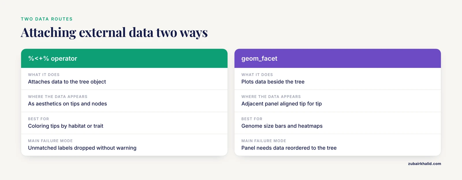
This is where most publication figures succeed or fail. Suppose you have per-taxon information in a data frame whose first column is label:

info <- data.frame(
    label          = c("Outgroup", "A", "B", "C", "D"),
    habitat        = c("root", "soil", "soil", "water", "water"),
    genome_size_mb = c(6.0, 5.1, 4.8, 3.2, 3.4)
)

Method 1 from the ggtree literature attaches this data to the tree object so its columns become available as aesthetics anywhere in the plot [1]:

p2 <- p %<+% info
p2 <- p2 +
    geom_tippoint(aes(color = habitat), size = 3) +
    geom_tiplab(aes(label = label), size = 3) +
    scale_color_brewer(palette = "Set1", name = "Habitat")

The %<+% operator matches rows of info to tips and internal nodes by label. The single most common ggtree failure follows from this matching: any row whose label does not exactly match a tip label is dropped silently, and any column you then reference in an aesthetic produces an error such as object 'habitat' not found or a plot missing the expected points. Before plotting, run info$label %in% tree$tip.label and confirm it returns TRUE for every row. Whitespace, case differences, and strain suffixes added by the tree-building pipeline are the usual culprits.

Method 2 plots data side by side with the tree, reordered to match the tree layout [1]:

p3 <- p2 +
    geom_facet(panel = "Genome size",
               data = info,
               aes(x = genome_size_mb),
               geom = geom_col, width = 0.6) +
    theme(legend.position = "bottom")

geom_facet creates an adjacent panel aligned tip-for-tip with the tree. For dense overlays such as heatmaps around circular trees, the companion Bioconductor package ggtreeExtra provides geom_fruit() layers that wrap around the tree, which is the standard pattern for genome and microbiome figures.

Step 8. Choose the layout and finalize the geometry

The layout argument controls the whole geometry:

ggtree(tree, layout = "circular")
ggtree(tree, layout = "unrooted")
ggtree(tree, layout = "daynight", open.angle = 30)
ggtree(tree, layout = "dendrogram", branch.length = "none")

branch.length = "none" ignores branch lengths and draws a cladogram with equal-length branches, which is appropriate when the tree is meant to convey topology only. open.angle creates a gap in circular layouts so tip labels have room. Rooting is a separate decision from layout: reroot with ape::root() before plotting if you want a specified outgroup at the base, because rerooting changes the interpretation of every node and should be fixed upstream, not adjusted cosmetically in the figure.

Step 9. Export at journal quality

ggsave("fig_tree.pdf", p3, width = 180, height = 120,
       units = "mm", useDingbats = FALSE)
ggsave("fig_tree.png", p3, width = 180, height = 120,
       units = "mm", dpi = 600)

Journals almost always prefer vector output (PDF, SVG, EPS) because it scales without loss. When a raster PNG or TIFF is required, 300 dots per inch is a common minimum for figures and 600 is safer for line art. Match the physical width and height in millimeters to the journal's column or page dimensions so that font sizes set in points in R survive to print at the intended size. Alongside the figure, save the processed tree itself with ape::write.tree(tree, file = "fig_tree.nwk") and save the R script and sessionInfo() output. Saving the ggtree object with saveRDS(p3, "fig_tree.rds") additionally preserves the embedded tree and annotation data inside the graphic object for later reuse [2].

Key options reference

Common mistakes and limitations

Label mismatches that fail silently. The %<+% operator drops unmatched rows without a warning. A single trailing space in a tip name makes an entire column vanish, and the first you hear of it is an object not found error in a later layer. Always verify labels with setequal(info$label, tree$tip.label) before plotting.

Support values in the wrong field. IQ-TREE and RAxML put support values in internal node labels, which is what treeio expects. Some pipelines instead append support values as :95 on internal branches, which parsers interpret as internal branch lengths. If your support labels plot as absurdly long branches or vanish entirely, inspect the raw Newick string in a text editor and check which position the numbers occupy.

Confusing a cladogram with a phylogram. Setting branch.length = "none" for visual convenience and then presenting the result as though it displays evolutionary distance misleads readers. Decide deliberately, and say in the caption whether the tree is scaled by substitutions per site or unscaled.

Rerooting as a cosmetic afterthought. Root position determines the direction of ancestor-to-descendant reading. Reroot on a justified outgroup, or use a documented midpoint approach, before any annotation layers are built, because node numbers change when the tree is rerooted and saved annotations will point at the wrong clades.

Overloaded figures. A tree with twelve annotation layers, four color scales, and three text sizes is unreadable at print size. Choose the two or three annotations that carry your biological argument. Web tools built around the same idea of data-driven annotation, such as tvBOT with its 26 supported annotation dataset types and its layer manager, enforce a similar discipline of organizing annotations as data layers rather than ad hoc drawing commands [8].

Ignoring uncertainty. For phylogenetic placement analyses, figures that show only the best placement hide the uncertainty that affects interpretation. The treeio-ggtree approach supports filtering placements and visualizing placement information on the final tree precisely so uncertainty is not lost [3]. If your analysis involves placement, show the uncertainty or explain why you did not.

Figure and text size mismatch. Font sizes in R are points at the size you export. Designing at default screen size and then scaling the PDF down in layout software shrinks the type below legibility. Export at final print dimensions from the start.

Undocumented methods. A tree figure is only as reproducible as its provenance. Applied guides across phylogenetics stress documenting the pipeline from data through inference, including software and settings [4]. Keep the tree file, the data frame, the script, and the saved ggtree object together in your repository.

Habit drift toward point-and-click tools. Interactive tools are useful for exploration, but manual adjustments made in a GUI are hard to reproduce exactly. Script everything, and use interactive adjustment only to discover parameter values you then write into the script.

Alternatives worth knowing

R and ggtree are not the only route to a finished tree figure, and knowing the alternatives helps you pick deliberately. tvBOT is a web application for visualizing, modifying, and annotating phylogenetic trees in which annotations are driven by a single table of data and rendered in real time, and it exports both publication-ready graphics and a JSON file that preserves the complete drawing state for later re-editing or reuse as a style template [8]. It is a strong choice when collaborators without R access need to annotate a tree.

In the Python ecosystem, T-REX wraps the ete3 toolkit to link trees with phenotypic data, run queries for entities of interest, and produce publication-ready figures, with particular attention to labeling large trees of strains for identification [9]. The baltic library, developed and used across decades of molecular epidemiology including the Ebola, Zika, and SARS-CoV-2 responses, parses BEAST Nexus, Newick, and Nextstrain JSON formats and plots through matplotlib, and it handles large BEAST posterior files in parallel [10]. If your figure lives inside a Python analysis pipeline, those tools avoid an R detour.

The choice is less about capability and more about workflow fit. If your whole analysis is already in R, if your data are Bioconductor objects, or if you need the tree, data, and figure to travel together as one reproducible artifact, ggtree is the shortest path [2].

Frequently Asked Questions

What makes a phylogenetic tree figure publication-ready?

It is a vector-format file at final print dimensions with legible fonts, a stated scale bar or a stated unscaled cladogram convention, support values where relevant, a declared root and outgroup, and a caption describing how the tree was inferred. Saving the underlying tree and data with the figure supports reproducibility [2].

Can ggtree read BEAST, IQ-TREE, and RAxML output directly?

Yes. treeio, the parser layer under ggtree, provides format-specific readers such as read.beast() for BEAST output and read.newick() for standard Newick files, and it retains metadata that generic readers would drop. Use the reader that matches your inference software.

How do I find internal node numbers for clade annotation?

Convert the ggtree object to a data frame with as.data.frame(p) and inspect the node and label columns for internal nodes, or use MRCA(p, "tipA", "tipB") to get the node number of the common ancestor of two tips. Node numbers are specific to each tree object, so always derive them from your own file.

Why do my external data columns disappear when I attach them?

The %<+% operator matches rows to tips by label, and unmatched rows are dropped without warning. Check that the first column of your data frame contains exactly the tip labels, including case and punctuation, with setequal(info$label, tree$tip.label).

What layout works best for a tree with hundreds of taxa?

Circular or fan layouts place long label lists efficiently around a ring, and ggtree is designed to handle large trees. Placement-focused workflows also demonstrate subtree extraction so you can show a relevant portion of a large reference tree with full annotation context [3].

Can I combine the tree with an alignment, heatmap, or bar chart?

Yes. ggtree's two data-mapping methods cover this: attach metadata directly to the tree with %<+%, or build side-by-side panels with geom_facet() after the package reorders the data to match the tree [1]. For circular layouts, use geom_fruit() from ggtreeExtra.

How do I export the figure at journal resolution?

Use ggsave() with explicit width and height in millimeters matched to the journal's column size, and save as PDF for vector output or as PNG or TIFF at 300 to 600 dpi for raster. Designing at final print size keeps point sizes in R correct on paper.

Is ggtree free, and where does it come from?

Yes. ggtree is open-source software distributed through Bioconductor, the project's official package repository, and it is documented alongside treeio and companion packages there [1]. Installation through BiocManager::install("ggtree") gets you the current release.

Sources

1. Two Methods for Mapping and Visualizing Associated Data on Phylogeny Using Ggtree.
2. Ggtree: a serialized data object for visualization of phylogenetic tree and annotation data
3. Scalable method for exploring phylogenetic placement uncertainty with custom visualizations using treeio and ggtree
4. Applied aspects of methods to infer phylogenetic relationships amongst fungi
5. SNPhylo: a pipeline to construct a phylogenetic tree from huge SNP data
6. Supermatrix and species tree methods resolve phylogenetic relationships within the big cats, Panthera (Carnivora: Felidae).
7. Characteristics, comparative genomics, and phylogenetic analysis of the chloroplast genome of Rosaplatyacantha.
8. Tree Visualization By One Table (tvBOT): a web application for visualizing, modifying and annotating phylogenetic trees
9. Tree Explorer (T-REX): Bridging Phylogenetic and Phenotypic Data for Enhanced Analysis and Interpretation
10. baltic: the Backronymed Adaptable Lightweight Tree vIsualisation Code