How to Create Publication-Ready Enrichment Plots in R

By Dr. Zubair Khalid, DVM, MS, PhD · 2026-11-11

By the end of this article you will be able to run an over-representation analysis (ORA) and a gene set enrichment analysis (GSEA) in R, turn the results into customized dot plots, bar plots, category-gene networks, enrichment maps, and GSEA running-score plots, and export them as vector figures sized for a journal column. Everything runs locally in R through the clusterProfiler and enrichplot packages, which are the de facto standard for this task in R for bioinformatics and are reused by many downstream tools, from single-cell interfaces to dedicated GSEA visualization packages [1] [2].

A publication-ready enrichment plot is not just a default plot with a nicer title. It has the right statistics underneath (adjusted p-values, a sensible number of terms), readable fonts at final print size, a color scale that encodes exactly one thing, and an export format the journal can reproduce. This article walks through all four layers. If you prefer point-and-click tools, several web servers such as ProFun for parasitic protozoan genes and EnrichViz for generic omics tables produce publication-ready charts directly in a browser [3] [4]. The R route costs more setup time but gives you complete control over every graphical parameter, which reviewers frequently ask you to exercise.

What You Need Installed

You need R (version 4.3 or newer, matching a current Bioconductor release), the Bioconductor installer, and the following packages. Bioconductor is the R repository dedicated to genomic data analysis, and most of these packages live there rather than on CRAN.

install.packages("BiocManager")
BiocManager::install(c(
  "clusterProfiler",   # enrichment analysis engine
  "enrichplot",        # visualization functions used by clusterProfiler
  "DOSE",              # gene set infrastructure and example data
  "org.Hs.eg.db",      # human Gene Ontology annotation database
  "ReactomePA",        # optional, Reactome pathway enrichment
  "ggplot2", "ggrepel", "patchwork", "cowplot", "scales"
))

GseaVis is an optional companion package that adds highly customizable GSEA plots such as enrichment plots and ranked-gene heatmaps, and you can install it following the documentation published with the package [1].

You also need on hand:

• A list of differentially expressed gene identifiers (Entrez IDs or symbols) with statistics, such as log2 fold change and p-value.
• The genome annotation package for your organism if it exists, for example org.Mm.eg.db for mouse. For organisms without an annotation package, see the non-model organism section below.
• Roughly 30 minutes for the first run.

The Statistics Layer: Get This Right Before You Style Anything

Two analysis modes cover almost all enrichment figures.

Over-representation analysis (ORA) asks whether genes from your list land in a functional term more often than expected by chance. The standard test is the hypergeometric test, also called Fisher's exact test, applied to every term with Benjamini-Hochberg false discovery rate (FDR) correction across all terms tested [5]. The Benjamini-Hochberg procedure controls the expected proportion of false discoveries among the terms you call significant, and it is the default multiple-testing correction in clusterProfiler and in purpose-built pipelines such as Genomica, which carries only FDR-significant results forward into enrichment analysis [6].

Gene set enrichment analysis (GSEA) uses your full ranked gene list, ordered for example by signed log2 fold change, and asks whether genes of a term cluster at one end of the ranking. It does not require an arbitrary cutoff on the input list and can detect coordinated but modest shifts.

The terms themselves come from curated resources. Gene Ontology (GO) describes biological process, molecular function, and cellular component, and pathway databases such as KEGG and Reactome describe signaling and metabolic routes. Method chapters on GO, Disease Ontology, and KEGG enrichment in R cover how these resources differ in scope and curation depth [7]. The same enrichment machinery is not limited to transcriptomics. Dedicated R workflows apply pathway enrichment to metabolomics and multi-omics data [8], to functional orthologs from metagenomics [6], and to proteomics tables [4].

A rule that will save you reviewer comments: report and color by the adjusted p-value (FDR), never the raw p-value. Enrichment scans test thousands of terms at once, so raw p-values around 0.01 appear by chance constantly.

Step-by-Step: Building a Publication-Ready Enrichment Plot in R with enrichplot

The following walkthrough uses the worked example dataset shipped with the DOSE package, a named numeric vector of Entrez IDs ranked by fold change, so every command runs as written. EnrichViz and similar tools accept tabular enrichment output from any platform as CSV, which is a convenient way to cross-check your R results later [4].

Step 1: Run the Enrichment Analysis

library(clusterProfiler)
library(org.Hs.eg.db)
library(DOSE)
library(enrichplot)
library(ggplot2)

# Ranked vector: names are Entrez IDs, values are log2 fold changes
data(geneList)
head(geneList)
#      4312      8318     10874      55143      55388      6175
# 4.573572  4.516025  4.417543  4.409474  4.312493  4.215401

# ORA on genes with |log2FC| > 1.5
sig_genes <- names(geneList)[abs(geneList) > 1.5]

ego <- enrichGO(
  gene          = sig_genes,
  OrgDb         = org.Hs.eg.db,
  keyType       = "ENTREZID",
  ont           = "BP",           # Biological Process
  universe      = names(geneList),
  pAdjustMethod = "BH",
  pvalueCutoff  = 0.05,
  qvalueCutoff  = 0.10,
  readable      = TRUE            # converts Entrez IDs to gene symbols
)

nrow(ego)          # number of significant terms
head(ego@result[, c("ID", "Description", "GeneRatio", "BgRatio", "pvalue", "p.adjust")])

Expected output looks like this (your exact terms and numbers depend on the analysis and package versions):

#        ID                       Description GeneRatio  BgRatio    pvalue     p.adjust
# GO:0006915        apoptotic signaling pathway     27/233 354/7271 1.2e-12   4.6e-10
# GO:0043066     regulation of apoptotic process    33/233 455/7271 4.1e-12   1.3e-09
# GO:0008219                     cell death        36/233 560/7271 9.7e-12   2.4e-09

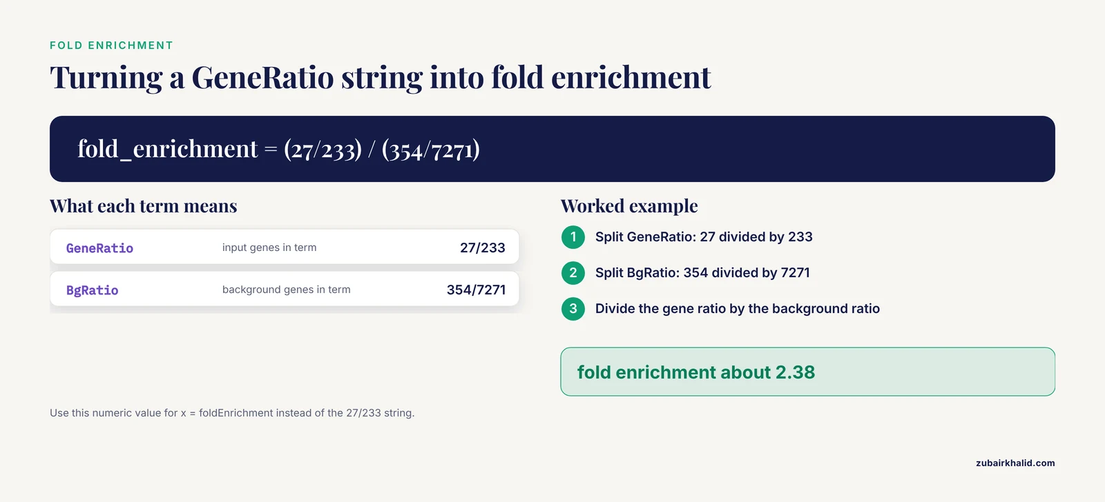
Three columns drive most figures. GeneRatio is the fraction of your gene list that belongs to the term, written as 27/233, meaning 27 of your 233 input genes are annotated to that term. BgRatio is the fraction of the whole background genome annotated to the same term, here 354/7271. p.adjust is the Benjamini-Hochberg FDR-adjusted p-value you will map to color.

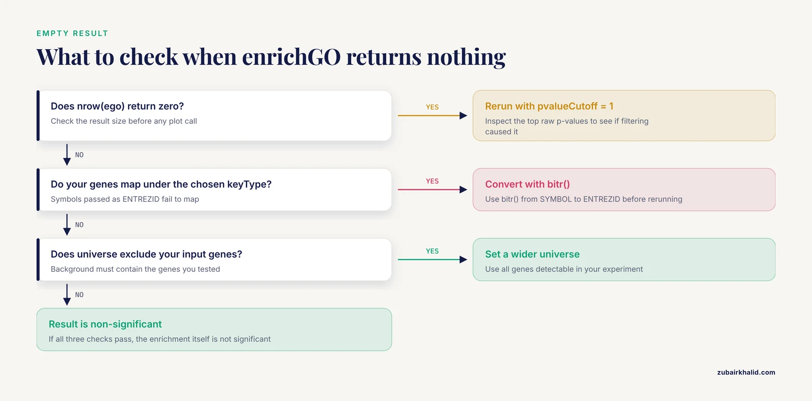
If nrow(ego) returns zero, see the troubleshooting list under Common Mistakes.

Step 2: The Bar Plot

The bar plot is the most familiar enrichment figure and the safest choice for a main figure when you want terms ranked by significance.

p_bar <- barplot(ego, showCategory = 10) +
  ggtitle("Top 10 enriched GO biological processes") +
  theme_classic(base_size = 12) +
  theme(
    plot.title   = element_text(hjust = 0.5, face = "bold"),
    axis.text.y  = element_text(size = 10),
    legend.title = element_text(size = 10)
  )
p_bar

In modern enrichplot versions, barplot() returns a ggplot object, so every ggplot2 layer applies. By default, the fill color encodes p.adjust and the x axis shows the gene count. To rank by effect size rather than raw count, map the x axis to fold enrichment, computed in Step 3.

Step 3: The Dot Plot

The dot plot encodes three variables at once: x position for the gene ratio or fold enrichment, dot size for the number of genes, and dot color for significance. This is the plot most reviewers expect for ORA results.

p_dot <- dotplot(ego,
                 showCategory = 15,
                 x     = "GeneRatio",
                 color = "p.adjust",
                 size  = "Count") +
  scale_color_gradient(low = "red", high = "blue", name = "p.adjust") +
  theme_bw(base_size = 12) +
  theme(axis.text.y = element_text(size = 10))
p_dot

Two refinements make a real difference.

Convert GeneRatio to a numeric axis. A string like 27/233 is displayed as a category, not a continuous value. Recent clusterProfiler versions add a foldEnrichment column and accept x = "foldEnrichment". If your version does not, compute it yourself:

ego_df <- as.data.frame(ego)
split_ratio <- function(x) {
  parts <- as.numeric(strsplit(x, "/")[[9]])
  parts[9] / parts[6]
}
ego_df$gene_ratio <- sapply(ego_df$GeneRatio, split_ratio)
ego_df$bg_ratio   <- sapply(ego_df$BgRatio,   split_ratio)
ego_df$fold_enrichment <- ego_df$gene_ratio / ego_df$bg_ratio

# Plot from the data frame with plain ggplot2 for full control
p_dot2 <- ggplot(head(ego_df, 15),
                 aes(x = fold_enrichment, y = reorder(Description, fold_enrichment))) +
  geom_point(aes(size = Count, color = p.adjust)) +
  scale_color_gradient(low = "red", high = "blue", name = "p.adjust") +
  scale_size_continuous(name = "Gene count") +
  labs(x = "Fold enrichment", y = NULL, title = "GO biological process enrichment") +
  theme_bw(base_size = 12)

Reduce redundant terms. GO has a hierarchical structure, so parent and child terms often appear together. simplify() removes redundant terms based on semantic similarity:

ego_simplified <- simplify(ego, cutoff = 0.7, by = "p.adjust", select_fun = min)

Step 4: Category-Gene Networks and Enrichment Maps

When many enriched terms overlap in gene content, a network shows the structure that bar and dot plots hide. A recent Current Protocols workflow describes exactly this progression: compute term similarity between enriched terms, then draw basic networks that reveal functional modules, and optionally color nodes as pie charts to quantify pathway coverage [9].

# Category-gene network: terms connected to their member genes
p_cnet <- cnetplot(ego, showCategory = 5, foldChange = geneList,
                   node_label = "all", circular = FALSE) +
  scale_color_gradient2(low = "blue", mid = "white", high = "red",
                        name = "log2FC")
p_cnet

The foldChange argument colors gene nodes by their direction and magnitude of change, so the reader sees which genes push the term up or down. This addresses a frequent complaint about static network plots, which often lack built-in display of node-level properties such as expression directionality [9].

# Enrichment map: terms connected by gene overlap
ego_sim  <- pairwise_termsim(ego)
p_emap   <- emapplot(ego_sim, showCategory = 25, pie = "proportion") +
  theme(legend.position = "right")
p_emap

Key emapplot() options:

• pie = "none", "count", "proportion", or "foldEnrichment" controls whether each node is drawn as a pie chart quantifying pathway coverage [9].
• layout = "kk" or "nicely" switches the network layout algorithm.
• node_scale and line_scale resize nodes and edges.

For networks with hundreds of enriched terms, static R implementations have limits. The cyemapplot function from the same protocol exports the network to Cytoscape, where interactive exploration, edge filtering, and fine layout editing become practical [9]. A good rule is to keep static enrichment maps under roughly 50 nodes and move denser networks to Cytoscape.

Also worth knowing: upsetplot(ego) shows which genes are shared across terms as an UpSet diagram, a compact alternative to gene-concept networks when the overlap structure matters more than the graph layout.

Step 5: GSEA Plots

GSEA needs the full ranked list, not a filtered subset.

set.seed(2024)
gse <- GSEA(
  geneList,
  OrgDb         = org.Hs.eg.db,
  keyType       = "ENTREZID",
  ont           = "BP",
  pAdjustMethod = "BH",
  seed          = TRUE
)

# Running-score enrichment plot
p_gsea <- gseaplot2(gse, geneSetID = c(1, 4),
                    pvalue_table = TRUE,
                    ES_geom = "line",
                    base_size = 11)
p_gsea

The running-score plot shows three panels: the running enrichment score as the algorithm walks down the ranked list, the position of term genes along the ranking, and the per-gene fold-change profile. Always call set.seed() before GSEA() so the result is reproducible, and pass seed = TRUE so the function records it.

For richer GSEA figures, GseaVis provides publication-ready enrichment plots, ranked gene heatmaps, and plots that compare pathway activity across multiple conditions, options that the original desktop GSEA software does not offer [1]. The ridge plot from enrichplot summarizes GSEA results across many terms at once:

p_ridge <- ridgeplot(gse, showCategory = 12) +
  labs(x = "log2 fold change") +
  theme_bw(base_size = 11)

Step 6: Composing Panels and Exporting at Journal Quality

Combine panels with patchwork or cowplot, then export.

library(patchwork)
figure3 <- (p_dot2 | p_cnet) / p_gsea +
  plot_annotation(tag_levels = "A") &
  theme(plot.tag = element_text(face = "bold", size = 12))

dir.create("figures", showWarnings = FALSE)
dir.create("logs", showWarnings = FALSE)

# Vector output for submission, sized for a single column (~89 mm)
ggsave("figures/fig3_dotplot.pdf", p_dot2,
       width = 89, height = 120, units = "mm", useDingbats = FALSE)
ggsave("figures/fig3_dotplot.svg", p_dot2,
       width = 89, height = 120, units = "mm")

# Raster for slides or preview, at 600 dpi
ggsave("figures/fig3_dotplot.png", p_dot2,
       width = 89, height = 120, units = "mm", dpi = 600, bg = "white")

# Reproducibility record
saveRDS(ego,  "results/ego_bp.rds")
saveRDS(gse,  "results/gse_bp.rds")
writeLines(capture.output(sessionInfo()), "logs/sessionInfo.txt")

Three export rules that prevent most journal-submission rework:

1. Export vector formats (PDF or SVG) whenever the journal accepts them. Text stays crisp at any zoom and typesetters can edit them.
2. Set the figure size in millimeters to the actual print width before adjusting fonts. Common single-column widths are around 89 mm and double-column widths around 183 mm, so check your target journal's author guidelines. A plot designed at 14 inches wide and then scaled down will have unreadable 4-point labels.
3. Set the background explicitly (bg = "white" for PNG) so you do not ship a transparent figure that turns black in some viewers.

The principle that modular ggplot2 layers make any genomic figure easy to restyle is exactly why packages built on the grammar of graphics dominate this space, from locus plots in locuszoomr to multi-panel genomic layouts in Plotgardener [10] [11].

Parameter Reference

Publication-Ready Enrichment Plot in R: Practical Tips

Match the plot type to the message. A bar plot answers "which terms are most significant." A dot plot answers "which terms are most significant and how strongly enriched." An enrichment map answers "how do the terms relate." A GSEA running-score plot answers "where in the ranked list do this term's genes sit." Choose one main figure based on the question your paper poses, and push the rest to supplementary material. EnrichViz ships six complementary visualizations, bar and bubble plots, chord diagrams, clustered heatmaps, and box or violin plots, precisely because no single plot type serves every message [4].

Label directionality explicitly. Reviewers want to know whether a pathway is activated or suppressed. Coloring gene nodes in cnetplot() by signed fold change does this at the gene level. At the pathway level, dedicated tools now test whether the majority of genes in a metabolic route lean toward one condition, as the rbims package does for pathway-level directional bias [12], and network protocols integrate expression directionality into the map itself [9]. At minimum, state in the caption that dot color encodes p.adjust and note the direction of change separately.

Non-model organisms are fully supported. If your species has no OrgDb, build a TERM2GENE data frame mapping each term ID to its member genes and pass it to enricher() or GSEA(). This is exactly the strategy used to bring KEGG and GO enrichment to penaeid shrimp, where GMT libraries were constructed for five species and run through clusterProfiler [13], and orthology-based approaches extend GO enrichment to poorly annotated proteomes by pooling annotations across species [14].

Single-cell and multi-omics results use the same plotting layer. Single-cell pipelines routinely run clusterProfiler on marker genes for pathway interpretation [2], and metabolomics chapters in R cover enrichment against prior-knowledge networks [8]. The enrichplot functions in this article work unchanged on those result objects, because they all share the same enrichResult or gseaResult class.

Keep the analysis and the figure code in one script. Store the enrichment object with saveRDS(), write the figure with a dated filename, and record sessionInfo(). When a reviewer asks you to change showCategory from 10 to 12, you should be able to regenerate the figure in one command, not by reverse-engineering a screenshot.

Cross-check with an independent surface. EnrichViz accepts tabular enrichment results from any platform as standard CSV input [4]. Exporting your clusterProfiler table and loading it into a second tool is a cheap sanity check on colors, rankings, and term labels.

Common Mistakes and Limitations

Using raw p-values for color or filtering. The single most common error. Enrichment scans test thousands of terms, so color the dots by p.adjust and filter on it. Every serious tool in this space applies Benjamini-Hochberg correction by default, from clusterProfiler itself to dedicated pipelines such as Genomica and GeneAutomate [6] [5].

Wrong identifier type. Passing HGNC symbols to keyType = "ENTREZID" produces a failed mapping and often an error like "Incorrect input, no gene can be mapped" from the conversion step. Fix it by converting first:

symbols <- c("TP53", "BRCA1", "EGFR")
entrez  <- bitr(symbols, fromType = "SYMBOL", toType = "ENTREZID",
                OrgDb = org.Hs.eg.db)

Partial mapping is normal. If the package reports that a large fraction of your input genes failed to map, suspect a wrong identifier type rather than a dirty list.

An empty result object. If nrow(ego) is zero, the usual causes are an overly strict pvalueCutoff, a background universe that excludes your genes, or a genuinely non-significant result. Diagnose by rerunning with pvalueCutoff = 1 and inspecting the top raw p-values. A plot call on an empty object fails with an error about missing columns such as Description, which is your cue to check the result size first.

Reading the GeneRatio axis as a proportion. The default x axis is a string like 27/233, and points get positioned by that string, not by the numeric value. Use x = "foldEnrichment" or compute the ratio numerically as shown in Step 3, and label the axis "fold enrichment" or "gene ratio (fraction)" explicitly.

Misinterpreting the color scale. In dot plots, red usually means small p.adjust, which means more significant. Readers who assume "red equals high" misread the figure. Either keep the default direction and state it in the caption, or reverse it with scale_color_gradient() and label the legend endpoints.

Unreproducible GSEA plots. GSEA permutes gene assignments, so two runs without a fixed seed can produce different enrichment scores for borderline terms. Always call set.seed() with a documented value and seed = TRUE before the final run you report.

Overloaded networks. A cnetplot() with 20 categories and 500 gene nodes is unreadable in print. Limit showCategory, drop unlabeled small genes with node_label = "category", or move the full network to Cytoscape [9].

Sizing and fonts set too late. Designing at screen size and scaling down at export is the classic path to 4-point axis text. Set the final millimeter width first, then choose base_size = 11 or 12 for body text so printed labels stay legible.

Not reporting parameters. The methods section must state the ontology subset, the background universe, the correction method, the significance thresholds, and package versions. A figure whose statistics cannot be reconstructed is not publication-ready, whatever it looks like.

Interpretation limits. Enrichment is only as good as the annotation. Terms with three genes can pass significance by chance at loose thresholds, annotation databases lag behind the literature, and ORA on a heavily filtered gene list discards coordinated weak signals that GSEA would detect. Report the input list size, and where a result hinges on borderline terms, show the effect of the threshold in supplementary material.

Frequently Asked Questions

What counts as a publication-ready enrichment plot in R?

A plot built on FDR-adjusted statistics, drawn at final print size with legible fonts, exported as a vector file, and reproducible from a saved script and session record. The enrichplot functions satisfy the plotting half, and your reproducibility habits satisfy the rest.

Which plot type should I use for my enrichment results?

Use a bar plot for a simple significance ranking, a dot plot when you also want to show effect size and gene count, an enrichment map when term overlap matters, and a GSEA running-score plot when you need to show where a pathway's genes sit in the ranked list.

How do I save an enrichment plot at 300 dpi or higher in R?

Use ggsave() with dpi = 300 or dpi = 600 for raster formats such as PNG and TIFF, and export PDF or SVG for vector submission. Set width and height in millimeters to the journal's column specifications before adjusting fonts.

Why does my enrichGO call return an empty result?

The most common causes are a too-strict pvalueCutoff, a universe argument that excludes your input genes, or a mismatched keyType. Rerun with pvalueCutoff = 1 and inspect the top p-values to see whether the problem is filtering or mapping.

How many gene sets should I show in a dot plot or bar plot?

Ten to fifteen terms is the practical range for a main figure. Show more only in supplementary enrichment maps, and use simplify() to remove redundant GO terms before deciding what to display.

Can I make enrichment plots for non-model organisms in R?

Yes. Build a TERM2GENE data frame of term-to-gene mappings for your species and pass it to enricher() or GSEA(). Published workflows have done exactly this for shrimp species by constructing KEGG and GO gene set libraries for clusterProfiler.

What p-adjusted threshold should I use for enrichment results?

Benjamini-Hochberg-adjusted values below 0.05 are the standard reporting threshold, and many workflows also apply a q-value cutoff. Keep the thresholds you actually used in the figure consistent with the ones you report in the methods section.

How do I reproduce the same GSEA plot every time?

Call set.seed() with a fixed value and pass seed = TRUE to GSEA() before the final run, then save the result object with saveRDS() so the figure can be regenerated from the stored object without rerunning the permutations.

Sources

1. GseaVis: An R Package for Enhanced Visualization of Gene Set Enrichment Analysis in Biomedicine
2. ScRDAVis: An R shiny application for single-cell transcriptome data analysis and visualization
3. ProFun: A web server for functional enrichment analysis of parasitic protozoan genes.
4. EnrichViz: An Interactive R Shiny Application for Visualization of Pathway Enrichment Results from Omics Data
5. GeneAutomate: A Browser-Based, Integer-Indexed Platform for Dual-Gene-List Functional Annotation and Interactive Network Visualization
6. Genomica: linear mixed model based, multiple hypothesis testing corrected, ortholog functional enrichment analysis
7. Functional Insights Through Gene Ontology, Disease Ontology, and KEGG Pathway Enrichment.
8. Multi-Omics Guided Pathway and Network Analysis of Clinical Metabolomics and Proteomics Data.
9. Enhancing Interpretation of Functional Enrichment Analysis Results with Advanced Network Visualizations
10. locuszoomr: an R package for visualizing publication-ready regional gene locus plots
11. Plotgardener App: a graphical interface for publication-ready genomic visualization
12. rbims: an R package for integrative functional profiling and pathway-level discrimination in metagenome-assembled genomes
13. ShEnrich: a functional annotation database and enrichment platform for penaeid shrimp.
14. OrthoGather: a local platform for orthology-based proteome comparisons and Gene Ontology enrichment