Publication-Quality Plots for Bioinformatics in Python
By Dr. Zubair Khalid, DVM, MS, PhD ·

By the end of this guide you will be able to take raw bioinformatics output, such as a FASTA file, a differential expression table, or a Newick tree, and turn it into a figure that survives peer review. You will set up a Python environment, configure matplotlib once so every figure matches journal formatting rules, build several complete plots step by step, export them as vector and high-resolution raster files, and check the results before submission.
Python has become a default language for python for bioinformatics work because analysis and visualization live in the same script. A large body of domain-specific tools now produces publication-quality output directly from sequencing data. SpliceV plots forward and back-splicing events with exon and single nucleotide coverage from RNA-seq experiments in a publication quality format [1]. svist4get generates publication-quality figures from genomic signal tracks through a command-line interface designed for automated pipelines [2]. This article shows you the general workflow underneath those tools so you can build figures for any analysis, not just the ones a packaged tool supports.
What You Will Build and What You Need
The walkthrough in this article produces four figures from real data formats:
- A scatter plot of GC content versus sequence length computed from a multi-FASTA file using Biopython.
- A volcano plot from a tabular differential expression result.
- A multi-panel composite figure sized to a journal column.
- A rendered phylogenetic tree using Bio.Phylo.
You need Python 3.10 or newer, a terminal, and about 2 GB of free disk space for the environment. Install the packages listed in Step 1 before you begin. Every code block runs as written if your input files match the described formats.
What Publication Quality Means for a Bioinformatics Figure
A publication-quality figure meets four requirements that reviewers, editors, and reproduction in print all depend on.
Vector or high-resolution output. Line art, such as plots, trees, and sequence diagrams, should be exported as vector files (PDF, SVG, or EPS) or as bitmaps at high dots-per-inch resolution. PConPy, a Python module for protein contact maps, explicitly advertises generation of publication-quality images in both vector and raster formats for exactly this reason [3]. svist4get likewise saves plots as vector images or high-resolution bitmaps [2].
Legible fonts at final size. A figure is shrunk to its final printed width, often a single column of roughly 8 to 9 cm or a double column of roughly 17 to 18 cm. An 8-point axis label that looks generous on a 20 cm screen figure becomes unreadable at 8 cm. You size the figure and fonts for the final printed dimensions, not for the screen.
Embedded, standard fonts. Text must be embedded in the exported file, and type 3 fonts (the matplotlib PDF default in older versions) are rejected by some publishers. Setting the font type to TrueType (type 42) avoids this.
Reproducibility. The figure must be regenerable from the script and the data. This is why command-line plotting tools are valued in pipelines. The tumor-normal quality control workflow published as part of the ngs-bits project computes QC metrics in C++ and relies on Python with matplotlib specifically for the plotting step, separating data processing from figure production [4]. aPEAch, an automated end-to-end pipeline for epigenomic and transcriptomic data, ships quality control reports and fragment size distribution plots as pipeline outputs so results can be re-executed and re-plotted with different parameters [5].
Step-by-Step Workflow for Publication-Quality Plots in Python
The following steps form a repeatable workflow. Steps 2 and 7 pay off across every figure you ever make, so do them once and reuse the file.
Step 1: Create a Dedicated Environment
Never plot in your base Python installation. A dedicated environment pins the versions that generated each manuscript figure.
conda create -n figures python=3.11
conda activate figures
pip install matplotlib pandas numpy biopython
Expected output (versions vary):
Successfully installed biopython-1.84 matplotlib-3.9.2 numpy-2.1.3 pandas-2.2.3Verify the install:
python -c "import Bio, matplotlib; print(Bio.__version__, matplotlib.__version__)"If you work in mass spectrometry, install spectrum_utils the same way. It is available for Python 3.6+ on PyPI and can be installed with conda, and it produces both publication-quality static figures and interactive spectrum plots for web pages [6].
Step 2: Set Global Style Defaults Once
Write a single style module, for example plotstyle.py, that every figure script imports. This is the single highest-leverage habit in the whole workflow.
# plotstyle.py
import matplotlib as mpl

mpl.rcParams.update({
    # Output
    "savefig.dpi": 300,
    "figure.dpi": 150,          # screen preview, export uses savefig.dpi
    "savefig.bbox": "tight",

    # Fonts: journal-appropriate size for a single-column figure
    "font.family": "sans-serif",
    "font.sans-serif": ["Arial", "Helvetica", "DejaVu Sans"],
    "font.size": 8,
    "axes.titlesize": 9,
    "axes.labelsize": 8,
    "xtick.labelsize": 7,
    "ytick.labelsize": 7,
    "legend.fontsize": 7,

    # Line weights: hairlines vanish at print size, defaults are too heavy
    "axes.linewidth": 0.75,
    "xtick.major.width": 0.75,
    "ytick.major.width": 0.75,
    "lines.linewidth": 1.0,

    # Text embedding for vector export
    "pdf.fonttype": 42,
    "ps.fonttype": 42,
    "svg.fonttype": "none",

    # Clean look
    "legend.frameon": False,
    "axes.spines.top": False,
    "axes.spines.right": False,
})
Then every figure script starts with:
import plotstyle  # applies rcParams on import
import matplotlib.pyplot as plt
Three settings here deserve explanation because they cause the most submission problems:
pdf.fonttypeandps.fonttypeset to 42 embed TrueType text instead of type 3 fonts, which keeps text editable in Illustrator and acceptable to most publishers.svg.fonttypeset to"none"keeps text as real text in SVG output rather than converting every glyph to a path, which makes the file unsearchable and bloated.savefig.dpiat 300 applies to everysavefigcall automatically, so you never accidentally ship a 100 DPI bitmap.
Step 3: Plot Sequence Statistics from a FASTA File with Biopython
This is the core of any Biopython tutorial approach to plotting: parse a standard format with Biopython, compute with plain Python, plot with matplotlib. Given a multi-FASTA file genes.fasta:
import plotstyle
import matplotlib.pyplot as plt
from Bio import SeqIO

ids, lengths, gc = [], [], []
for record in SeqIO.parse("genes.fasta", "fasta"):
    seq = str(record.seq).upper()
    ids.append(record.id)
    lengths.append(len(seq))
    gc.append((seq.count("G") + seq.count("C")) / len(seq) * 100)

fig, ax = plt.subplots(figsize=(3.5, 2.5), constrained_layout=True)
ax.scatter(lengths, gc, s=10, alpha=0.6, color="#2166ac", edgecolors="none")
ax.set_xlabel("Sequence length (nt)")
ax.set_ylabel("GC content (%)")
fig.savefig("gc_content.pdf")
fig.savefig("gc_content.png")
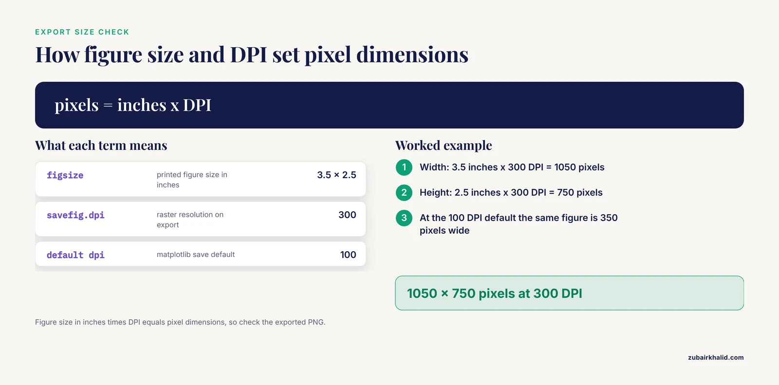
Expected result: a compact scatter plot where a PDF opens in any viewer at true print size (3.5 by 2.5 inches) and the PNG is a 300 DPI bitmap at 1050 by 750 pixels. Figure size in inches times DPI equals pixel dimensions, so check with:
from PIL import Image
img = Image.open("gc_content.png")
print(img.size)  # (1050, 750)
constrained_layout=True automatically adjusts axes and labels so nothing is clipped, replacing the older tight_layout() call. The figsize=(3.5, 2.5) matches a single journal column, which is the point of the whole exercise.
Step 4: Build a Volcano Plot from Differential Expression Results
Given de_results.tsv with columns gene, log2fc, and padj:
import plotstyle
import matplotlib.pyplot as plt
import pandas as pd
import numpy as np

df = pd.read_csv("de_results.tsv", sep="\t")
df["neg_log10_p"] = -np.log10(df["padj"].clip(lower=1e-300))

sig = (df["padj"] < 0.05) & (df["log2fc"].abs() > 1)

fig, ax = plt.subplots(figsize=(3.5, 2.8), constrained_layout=True)
ax.scatter(df.loc[~sig, "log2fc"], df.loc[~sig, "neg_log10_p"],
           s=5, color="0.75", edgecolors="none", rasterized=True)
ax.scatter(df.loc[sig, "log2fc"], df.loc[sig, "neg_log10_p"],
           s=6, color="#b2182b", edgecolors="none", rasterized=True)
ax.axhline(-np.log10(0.05), lw=0.75, color="black", ls="--")
ax.axvline(1, lw=0.75, color="black", ls="--")
ax.axvline(-1, lw=0.75, color="black", ls="--")
ax.set_xlabel("log2 fold change")
ax.set_ylabel("-log10 adjusted p-value")
fig.savefig("volcano.pdf")
Two details make this publication quality rather than merely plotted:
rasterized=Trueon the scatter layers keeps tens of thousands of points as a bitmap inside an otherwise vector PDF. Without it, a 30,000-point scatter plot produces a PDF of tens of megabytes that stalls reviewers' PDF viewers.- The thresholds (adjusted p-value below 0.05, absolute log2 fold change above 1) are drawn on the figure and stated in the axis labels region of your methods, so the reader never has to guess the cutoffs.
Step 5: Assemble a Multi-Panel Figure at Journal Dimensions
Journals almost never accept separately submitted panels that the typesetter will assemble for you. Build the composite yourself so panel labels and spacing are under your control.
import plotstyle
import matplotlib.pyplot as plt
import matplotlib.gridspec as gridspec

fig = plt.figure(figsize=(7.2, 4.0), constrained_layout=True)
gs = gridspec.GridSpec(2, 2, figure=fig)

ax_a = fig.add_subplot(gs[0, 0])
ax_b = fig.add_subplot(gs[0, 1])
ax_c = fig.add_subplot(gs[1, :])

# ... plot into ax_a, ax_b, ax_c ...

for ax, label in zip([ax_a, ax_b, ax_c], ["a", "b", "c"]):
    ax.text(-0.12, 1.05, label, transform=ax.transAxes,
            fontsize=10, fontweight="bold", va="top")
Panel labels go outside the axes using transform=ax.transAxes, and they move with the panel if you rearrange the grid later. A 7.2 inch width corresponds to a double-column figure. The free space you see between panels in constrained_layout output is normal and much safer than manual subplots_adjust tweaking.
Step 6: Draw a Phylogenetic Tree with Bio.Phylo
Biopython's tree module renders Newick files through matplotlib, so the same style settings apply:
import plotstyle
import matplotlib.pyplot as plt
from Bio import Phylo

tree = Phylo.read("tree.nwk", "newick")

fig = plt.figure(figsize=(3.5, 5.0), constrained_layout=True)
ax = fig.add_subplot(1, 1, 1)
ax.axis("off")
Phylo.draw(tree, axes=ax, do_show=False)
fig.savefig("tree.pdf")
do_show=False prevents the interactive window from blocking a batch script. For larger or more decorated phylogenies, the ETE Toolkit is a dedicated Python package for annotating and visualizing large phylogenies, and it is one component of an integrated ecosystem with TreeProfiler and PhyloCloud built for phylogenomic datasets that have outgrown ad hoc plotting [7].
Step 7: Export Vector and Raster Files Correctly
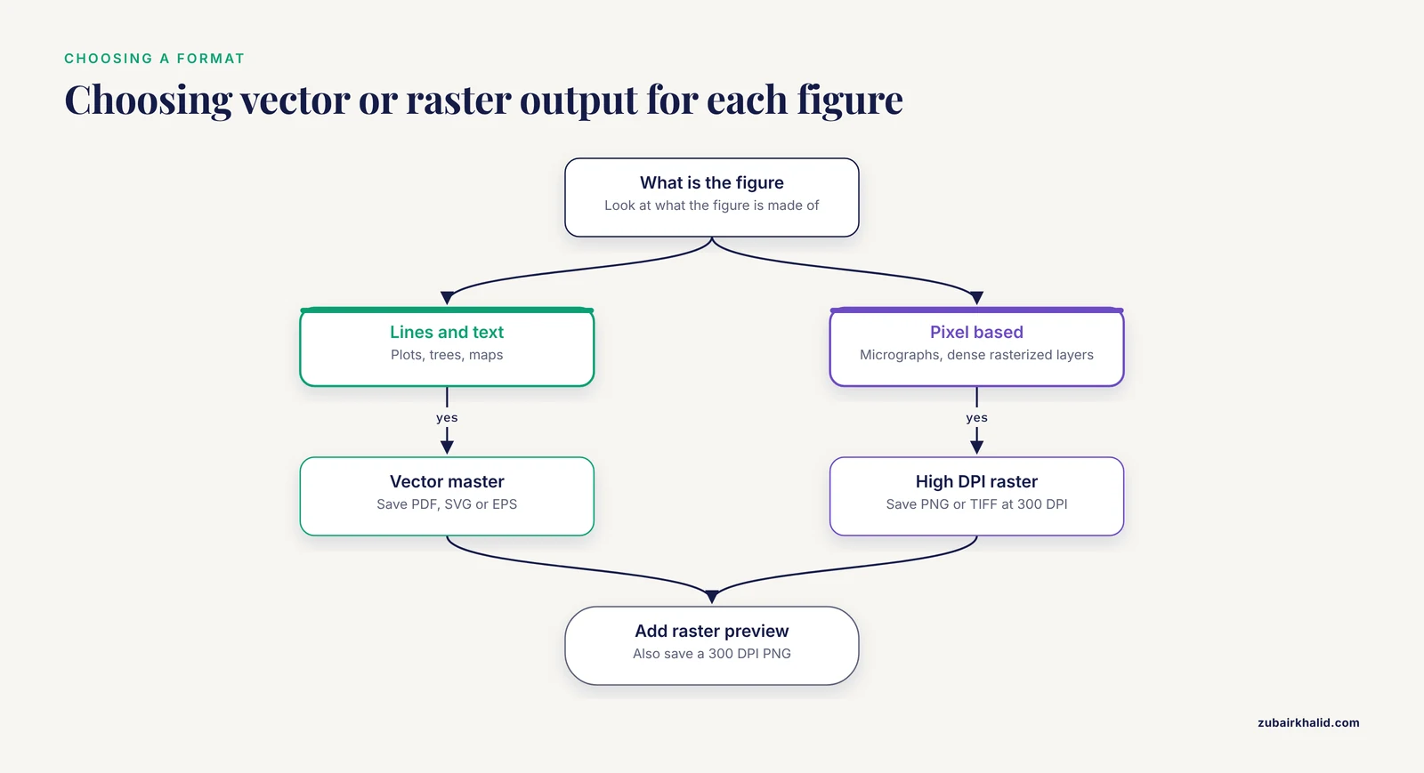
Export both a vector master and a raster preview for every figure:
fig.savefig("figure1.pdf")          # vector master for submission
fig.savefig("figure1.png", dpi=300) # raster preview and slide use
fig.savefig("figure1.svg")          # editable vector, if the journal asks
fig.savefig("figure1.tiff", dpi=300)  # some journals require TIFF
The following table summarizes the settings that control export quality.
| Setting | Where it applies | Recommended value | Why it matters |
|---|---|---|---|
figsize | Figure creation | Final printed size, e.g. (3.5, 2.5) inches | Fonts scale with figure size, so wrong size means wrong font size |
savefig.dpi | All raster exports | 300 for photos and heatmaps | Lower values blur in print |
pdf.fonttype / ps.fonttype | PDF and EPS export | 42 (TrueType) | Type 3 fonts are rejected by some publishers |
svg.fonttype | SVG export | "none" | Keeps text editable and searchable instead of paths |
rasterized | Individual artists | True on dense scatter or heatmap layers | Keeps vector text and axes with a small file size |
bbox_inches | savefig | "tight" | Prevents clipped labels without manual padding |
constrained_layout | Figure creation | True | Prevents overlapping labels automatically |
A practical rule for choosing between formats: vector for anything made of lines and text (plots, trees, maps), high-DPI raster for anything genuinely pixel-based (micrographs, dense rasterized layers).
Step 8: Verify the Figure Before Submission
Run this five-point check on every figure:
- Open the PDF at 400 percent zoom. Vector line art stays sharp at any zoom. If edges pixelate, something was rasterized unintentionally.
- Print the figure at final size on plain paper. If you cannot read the axis ticks at arm's length, neither can a reviewer.
- Check that fonts are embedded. In a PDF viewer, look at document properties for the font list, or run
pdffonts figure1.pdfand confirm embedded subsets rather than type 3 fonts. - Convert the figure to grayscale. If two conditions become indistinguishable, change the palette. Shape and position cues (different markers, direct labeling) survive grayscale better than color alone.
- Re-run the script from a clean checkout of your repository and confirm the identical figure is produced. If it is not, the figure depends on state that is not recorded anywhere.
Python Packages That Handle Specialized Bioinformatics Plots
Generic matplotlib covers a lot, but several plot types in biology are specialized enough that a dedicated package saves days of work. Each of the following is built on Python and produces publication-quality output.
| Package | Plot type | Input data | Notable workflow feature |
|---|---|---|---|
| SpliceV [1] | Splicing, sashimi-style coverage | RNA-seq splice junction and coverage data | Plots forward and back-splicing at exon and nucleotide level |
| SplicePlot [8] | Sashimi, hive, structure plots | BAM reads plus VCF genotypes | Command-line tool showing genotype-dependent splicing |
| svist4get [2] | Genomic signal tracks | Mapped read coverage tracks | CLI tool made for automated pipeline use |
| CoMut [9] | Comutation (oncoprint-style) | Arbitrary mutation and clinical data | Object-oriented API, also usable in Google Colab |
| spectrum_utils [6] | Mass spectra | Standard mass spectrometry formats | Static publication figures plus interactive web plots |
| SimPlot++ [10] | Sequence similarity plots | Aligned sequences | 63 nucleotide and 20 amino acid distance models |
| PConPy [3] | Protein contact and distance maps | Protein structure data | Vector and raster output, flexible contact definitions |
| GENOVIS [11] | Manhattan, PCA, admixture, ROH plots | Population genetics outputs | Both CLI and GUI interfaces |
| ETE Toolkit [7] | Phylogenetic trees with annotation | Tree files plus metadata | Scales to large phylogenies |
| sortscore [12] | Variant effect heatmaps | Sort-seq / MAVE counts | Scoring plus heatmap visualization in one package |
| SpotSweeper-py [13] | Spatial QC plots | Spatial transcriptomics (scverse) | Plotting utilities for flagged outliers |
| seqme [14] | Sequence design diagnostics | Generative model outputs | Metrics plus visualization in one library |
A few of these deserve workflow-level comment.
For splicing visualization, choose by input format and population context. SplicePlot takes mapped RNA-seq reads in BAM format and genotype data in VCF format and outputs publication-quality Sashimi plots for investigating splicing quantitative trait loci at a population level [8]. SpliceV goes further into regulation-oriented views, plotting all relevant forward- and back-splice data with exon and single nucleotide level coverage and overlaying predicted RNA binding protein sites and repetitive elements [1]. If your figure needs to show genotype-dependent splice usage, the BAM plus VCF path in SplicePlot is the direct route.
For genomic tracks, svist4get fills a specific niche: many genome browser tools produce interactive web views, but svist4get is a command-line application built for automated, reproducible generation of publication-ready track figures, aggregating several tracks on a single plot with transcriptome annotation, customizable through configuration files and a Python API [2]. It installs from PyPI and runs as part of a console pipeline.
For cohort genomics, CoMut creates highly customizable publication-quality comutation plots from arbitrary user data, including categorical data, continuous data, and sample-relationship information, as a stand-alone object-oriented Python package [9]. GENOVIS addresses the other end of the usability spectrum, offering both command-line and graphical interfaces for six core population genetics visualizations including SNP density heatmaps, 3D PCA, admixture barplots, and Manhattan plots, motivated by the difficulty researchers without a bioinformatics background face in producing customizable figures [11].
For mass spectrometry, spectrum_utils wraps reading standard file formats, processing spectra, and visualization in a high-level API so that common script functionality does not need to be reimplemented, and its visualization layer produces publication-quality figures as well as interactive plots [6].
Two newer tools round out the picture for specific data modalities. SpotSweeper-py brings spatially-aware quality control metrics for spatially resolved transcriptomics into the Python scverse ecosystem, with plotting utilities included for quick visualization of flagged outliers, addressing the earlier limitation that the original SpotSweeper existed only in R [13]. seqme provides metrics and visualization functions for evaluating biological sequence design from generative models across DNA, RNA, peptides, and proteins [14]. Finally, the Plotgardener App shows where the field is heading on accessibility: it wraps the code-driven Plotgardener genomic visualization package in a desktop graphical interface with a Python parser that keeps the interface synchronized with the underlying package, so publication-ready genomic plots can be made without programming experience [15].
Publication-Quality Plot Tips from Working Pipelines
These tips come from patterns visible across the domain-specific tools above and from daily practice.
Put plotting in its own step. The ngs-bits QC workflow computes metrics in one set of tools and plots in another, with an intermediate structured output connecting them [4]. Decoupling analysis from plotting means you can re-plot without re-running a 12-hour alignment, and it forces your figure to depend on a saved data file rather than on in-memory state. aPEAch follows the same philosophy by emitting all intermediate files alongside its plots so the analysis can be re-executed with different parameters or representations [5].
Prefer the packaged tool when the plot type is standard. A hand-rolled Manhattan plot or Sashimi plot will cost you a week and still miss layout conventions that GENOVIS, SplicePlot, or svist4get already encode. Reserve custom matplotlib work for the figure no package supports.
Drive everything from configuration, not from edited files. svist4get exposes customization through configuration files and a Python API rather than through manual figure editing [2]. The equivalent habit in your own scripts is keeping figure dimensions, thresholds, and color assignments in one config block at the top of the script rather than scattered through plotting calls.
Keep the CLI path alive even if you plot interactively. Every tool in the table with a command-line interface (svist4get, SplicePlot, GENOVIS, spectrum_utils via conda) can be called from a workflow manager. If you build figures only in a notebook session, they stop being reproducible the day the notebook state is lost.
Rasterize dense layers, vectorize everything else. This one setting, rasterized=True on heavy scatter or heatmap layers, is the difference between a 2 MB submission-ready PDF and a 200 MB file that crashes the submission system.
Match panel sizes exactly across figures in a manuscript. If Figure 1a and Figure 2a both show a scatter plot of the same physical width, give both the same figsize and font sizes. Readers notice mismatched panel typography immediately, and it suggests careless work.
Test the figure the way the reader sees it. Grayscale printout, small size, and a laptop PDF viewer catch problems that a 4K monitor hides.
Common Mistakes and Limitations
These are the mistakes that generate revision requests and wasted days, in rough order of frequency.
Exporting screen-resolution PNGs. The single most common error. matplotlib defaults to 100 DPI on save. A 3.5 inch figure exported this way is 350 pixels wide and turns to mush in print. Always confirm the pixel dimensions of your exported file equal inches times your intended DPI.
Sizing figures for the screen. A figure made at 12 by 8 inches with 10-point fonts, shrunk by the journal to 8.5 cm, ends up with effectively unreadable 4-point text. Set figsize to the final printed dimensions and choose fonts between 6 and 9 points.
Using default matplotlib colors and fonts. The default matplotlib font is DejaVu Sans, and default colors like the original tab-blue cycle look unmistakably like unpolished matplotlib. Journals do not reject figures for this, but reviewers notice. Setting Arial or Helvetica with the rcParams block above fixes both at once.
Type 3 fonts in PDFs. Older matplotlib defaults embed type 3 fonts in PDF and EPS output, which some publishers reject because the glyphs render poorly. pdf.fonttype: 42 prevents this before it happens.
Letting text become paths in SVG. With svg.fonttype left at its default, matplotlib converts all text to vector paths. The figure looks fine but the text is not searchable, not accessible to screen readers, and hard for co-authors to correct.
Hand-editing exported figures. Moving a label or changing a color in Illustrator, saving over the PDF, and never updating the script silently breaks reproducibility. Every manual edit you make is an edit the script will undo the next time it runs. If a label genuinely needs fixing, fix the script.
Overplotting without rasterization. Single-cell datasets routinely involve hundreds of thousands of points. A fully vector scatter plot of that size produces enormous files. Either rasterize the data layer or subsample and report that you did.
Color choices that fail in grayscale or for colorblind readers. The old rainbow (jet) colormap distorts perceived magnitude and fails grayscale conversion. Perceptually uniform colormaps such as viridis and cividis, or well-designed diverging palettes, are the standard expectation now. Add direct labeling or marker shape differences when color encodes your key comparison.
Inconsistent thresholds and units between panels and text. If the volcano plot uses adjusted p-value below 0.05 and the methods text says nominal p-value below 0.05, a careful reviewer will flag it. State every cutoff in the figure itself where possible.
Not version-controlling the figure code. A figure whose generating script exists only on one lab machine, next to a conda environment nobody documented, cannot be reproduced after a student leaves. Commit the script, the input data reference, and the environment file (for example environment.yml) together.
A limitation of Python plotting itself. matplotlib controls individual graphical elements precisely but has no native concept of biological semantics, which is exactly why the domain-specific packages above exist. Expect to combine them: parse and process with Biopython or pandas, plot specialized views with a domain package, and assemble final composites with matplotlib. Also note platform differences, for example svist4get is implemented in Python 3 and runs on Linux [2], so check operating system support before standardizing a lab workflow on any single tool.
Frequently Asked Questions
What DPI should I use for publication-quality figures?
Use 300 DPI for raster images as a widely accepted baseline for print, and vector formats (PDF, SVG, EPS) for line art whenever the journal accepts them, in which case DPI applies only to any rasterized layers inside the figure. Set this once in rcParams with savefig.dpi so you never export accidentally at the 100 DPI default.
Should I submit PDF, SVG, or PNG figures?
Submit vector files (PDF or EPS) for plots, trees, and line art, and high-resolution raster (PNG or TIFF) only for genuinely pixel-based content such as microscopy images. Vector files stay sharp at any scale and keep text embedded, which is why tools like PConPy and svist4get emphasize both vector and high-resolution bitmap export options [3] [2].
Do I need Biopython to make publication-quality plots in Python?
No, Biopython is not required for plotting itself, matplotlib does the rendering. Biopython earns its place by parsing biological formats, such as FASTA, GenBank, and Newick, into objects you can plot directly, and Bio.Phylo renders trees straight onto matplotlib axes as shown in Step 6.
How do I make my matplotlib figures match journal column widths?
Set figsize in inches to the final printed size, typically about 3.5 inches for a single column and about 7.2 inches for a double column, then set font sizes between 6 and 9 points in rcParams. Check your target journal's author guidelines for exact dimensions, since they vary between publishers.
What is the fastest way to make a Sashimi plot or genomic track figure?
Use a dedicated tool instead of building one from raw matplotlib. SplicePlot produces publication-quality Sashimi plots from BAM reads and VCF genotype data [8], SpliceV plots splice junctions with exon and nucleotide-level coverage [1], and svist4get renders genomic signal tracks as publication-quality figures from the command line [2].
How do I fix the warning that font family Arial was not found?
Either install the font on your system, list a fallback such as Helvetica or DejaVu Sans in font.sans-serif, or switch the whole figure to DejaVu Sans. matplotlib substitutes an available font and keeps plotting, so the warning is not fatal, but the substituted font may differ from your submitted figures unless you control the fallback order.
How do I keep figures reproducible across machines and collaborators?
Pin your environment (export environment.yml from conda), commit the plotting scripts and any configuration files to version control, have scripts read input data from files rather than notebook state, and follow the pipeline pattern of separating data processing from plotting with intermediate files [4]. Re-running the script from a clean checkout should regenerate the identical figure.
Which Python packages handle specialized bioinformatics plot types?
Use CoMut for comutation plots from arbitrary cohort data [9], spectrum_utils for mass spectra [6], GENOVIS for population genetics plots such as Manhattan and admixture barplots [11], ETE Toolkit for annotated phylogenies [7], sortscore for variant effect heatmaps [12], and SpliceV or SplicePlot for splicing visualizations [1] [8]. Reach for generic matplotlib when no package covers your figure type.
Sources
- SpliceV: analysis and publication quality printing of linear and circular RNA splicing, expression and regulation.
- svist4get: a simple visualization tool for genomic tracks from sequencing experiments.
- PConPy--a Python module for generating 2D protein maps.
- A comprehensive quality control workflow for paired tumor-normal NGS experiments.
- aPEAch: Automated Pipeline for End-to-End Analysis of Epigenomic and Transcriptomic Data.
- spectrum_utils: A Python Package for Mass Spectrometry Data Processing and Visualization.
- An Integrated Ecosystem for Analysis and Visualization of Large-Scale Phylogenomic Data Combining ETE Toolkit, TreeProfiler, and PhyloCloud for Scalable Phylogenomic Analysis.
- SplicePlot: a utility for visualizing splicing quantitative trait loci.
- CoMut: visualizing integrated molecular information with comutation plots.
- SimPlot++: a Python application for representing sequence similarity and detecting recombination.
- GENOVIS: a Python package for the visualization of population genetic analyses.
- sortscore: Sort-seq MAVE scoring and visualization using Python.
- Spotsweeper-py: spatially-aware quality control metrics for spatial omics data in the Python ecosystem.
- seqme: a Python library for evaluating biological sequence design from generative models.
- Plotgardener App: a graphical interface for publication-ready genomic visualization.