Provenance Capture in Bioinformatics: What to Record
By Dr. Zubair Khalid, DVM, MS, PhD ·
Provenance capture in bioinformatics is the systematic recording of the inputs, software versions, parameters, and execution conditions that produced a data file, written in a form a machine can parse and a reviewer can audit. A complete record answers seven questions for every output: which data came in, which reference was used, which code and versions ran, which settings were applied, on which computer, in what order, and who or what triggered the run.
This matters because genomics pipelines chain dozens of tools, and every link can silently break reproducibility. A case study that rebuilt a complex genomic workflow under three different workflow systems found that each system carried implicit assumptions about its execution environment, and those assumptions produced documentation too thin to re-execute the workflow reliably [1]. The consequences reach far beyond a failed rerun. Regulatory communication for precision medicine now expects standardized reporting of computational methods alongside wet-lab procedures [2]. Large consortia capture reference versions, software versions, and parameters for every processed experiment so that thousands of datasets stay comparable [3]. Public health genomic surveillance depends on sample context recorded next to sequence data, because a genome without its context cannot support a response decision [4]. Provenance capture is the discipline that makes all three possible.
What Is Provenance Capture in Bioinformatics?
In computing, provenance is the documented history of a data product, expressed as entities (the files, genomes, and containers involved), activities (the runs, transformations, and analyses), and agents (the people, pipelines, and organizations responsible). Capture means recording that history automatically while the work happens, rather than reconstructing it afterward from memory. The foundation is W3C PROV, a World Wide Web Consortium data model that represents entities, activities, agents, and the relationships between them, such as "used" and "wasGeneratedBy" [5].
Bioinformatics adopted provenance-aware execution early through workflow middleware, while fields built on distributed, heterogeneous clinical software started later, a contrast drawn in the learning health system literature where bioinformatics practice is cited as the model to follow [6].
Provenance is often confused with four neighboring ideas. The distinctions matter because each fills a different gap, and having one does not cover the others.
| Term | What it records | Typical form | What breaks without it |
|---|---|---|---|
| Provenance | Entities, activities, and agents linking inputs to outputs | W3C PROV graph, RO-Crate, BioCompute Object | You cannot say how a result was produced |
| Metadata | Properties of a dataset itself, such as tissue and platform | Structured fields, ontology terms | Data cannot be found or interpreted |
| Run log | Console output of one execution | Plain text file | Failures cannot be diagnosed |
| Version control | Changes to source files over time | Git history | Code changes cannot be traced |
| Reproducibility | The ability to re-obtain a result | Re-execution test | Results cannot be verified by others |
What to Record: The Core Checklist
Whatever standard you choose, the same seven classes of information recur. Record all seven and any output can be traced end to end. Skip one and a gap opens that no downstream tool can repair.
1. Input Data and Sample Context
Every input file needs an identity that survives a copy: a checksum, a fixed-length fingerprint computed with an algorithm such as SHA-256, plus a source accession (the stable identifier a repository assigns) when the file came from a repository. Beyond files, record the biological and epidemiological context of each sample: host species, tissue, collection date and location, extraction and library preparation methods, and laboratory results. In pathogen genomics this contextual data is what turns a sequence into public health evidence, and the Mpox contextual data specification was developed precisely because such metadata arrives unstructured, variable in format and terminology, and demands laborious manual cleanup before it can be used [4]. Large archives face the same requirement at scale, which is why the TCGA Expedition scripts download, extract, harmonize, version, and store both data and metadata for a corpus exceeding 1.2 petabytes [7].
2. Reference Genomes and Annotations
Record the exact assembly accession and version, the annotation release, and the derived files your pipeline actually consumed, such as the aligner index. FASTA and GFF have carried sequence and feature positions for over 25 years, yet assemblies are updated and re-annotated without systematic documentation of what changed, so different annotation versions cannot be computationally compared and version control is left to researchers juggling filenames, directories, and README files [8]. An index built with bwa index is a function of the exact FASTA bytes, which is why the reference checksum belongs in the record next to the accession.
3. Software, Containers, and Versions
For every tool, record the name, version, build, and installation method. Containers make this tractable: a container image packages a tool with its libraries, and a digest is the registry's immutable content hash for that image. Record the digest rather than a mutable tag, because a tag can be repointed to different content at any time. ENCODE's uniform processing pipelines capture all data files, reference genome versions, software versions, and parameters, and distribute the code as Docker images and WDL (Workflow Description Language) so that any laboratory can run the same stack [3]. Package environments deserve the same treatment, for example a pinned conda environment file or a lockfile committed beside the code.
4. Parameters and Configuration
Record every flag, threshold, and value, including the ones left at defaults, because defaults change between releases. Record random seeds for any stochastic step. Resource settings such as thread counts belong here too, since some tools change output ordering or chunking when parallelism changes. In practice these values live in a versioned configuration file, which the workflow engine then echoes into the provenance record.
5. Execution Environment and Resources
Record the operating system, the workflow engine (the software that executes multi-step pipelines and manages dependencies) and its version, the cluster queue or cloud region, CPU count, memory, disk, and wall-clock time. The DataLad-based FAIRly big framework shows the target state: machine-actionable provenance records that let a research outcome be retraced and re-executed independently of the original computing infrastructure, demonstrated at the scale of the UK Biobank dataset [9].
6. Workflow Structure and Step-Level Lineage
Record three layers: the abstract workflow (the plan), the planned steps with their dependencies, and the concrete execution (what actually ran, in what order, with which files). CWLProv was designed as a standards-based format that captures this hierarchy and packages it so the workflow is fully re-executable with domain-specific information attached [10]. Workflow Run RO-Crate generalizes the idea across engines. RO-Crate (Research Object Crate) is a convention for packaging data, metadata, and provenance in a folder with a machine-readable description, and the Workflow Run extension captures execution provenance at different levels of granularity while bundling inputs, outputs, and code together [11].
7. Outputs, Agents, Errors, and Timestamps
Record output files with checksums, creation timestamps, and the responsible agent, whether a person, an automated pipeline, or an institution. Failures belong in the record as well. The BioCompute framework defines a dedicated error domain alongside its provenance, usability, and execution domains, so a report can state what ran and also what went wrong and how it was handled [2].
How Provenance Capture Works, Step by Step
Step 1, authoring time. Write the workflow in a declarative language such as CWL (Common Workflow Language) or WDL, declare inputs and types, pin containers, and commit the code to version control. Anything declared here becomes part of every later record.
Step 2, run time. The workflow engine observes execution and writes the activity graph: which step consumed which file, produced which output, under which container. Running a CWL workflow with cwltool and provenance recording enabled produces a CWLProv research object, a folder that bundles the workflow definition, the W3C PROV graph, and every input and output file [10]. Other engines write Workflow Run RO-Crate instead, and the model is implemented across six workflow systems, which makes runs from heterogeneous engines directly comparable [11].
Step 3, packaging. The run record is bundled with code and data into a shareable artifact: a research object crate, or a BioCompute Object for standardized reporting. BioCompute Objects encapsulate tools, platforms, datasets, and workflows in a FAIR-compliant structure (FAIR stands for Findable, Accessible, Interoperable, Reusable), and cloud platforms including Galaxy and the Cancer Genomics Cloud support generating them for users [12].
Step 4, sharing and query. Publish the package with a persistent identifier. Because the content is a PROV graph, questions become queries: which inputs fed this output, which agent ran that step, which reference version was used. Work in simulation biology shows the same graph can link a model to its ancestors, so a family of 19 Wnt signaling models was related through shared entities and activities such as building, calibrating, and validating [5].
Standards You Will Meet
W3C PROV
The graph model underneath most workflow provenance formats, defining entities, activities, agents, and relationships such as used and wasGeneratedBy [5]. Learn to read a PROV graph and every workflow provenance format becomes legible.
CWLProv and Workflow Run RO-Crate
CWLProv packages a CWL run as a research object with PROV inside, built from best practices identified across the workflow sharing literature [10]. Workflow Run RO-Crate extends RO-Crate and Schema.org to capture run provenance at multiple granularities and is implemented by several workflow management systems [11]. Choose these when the goal is a re-executable bundle.
BioCompute Objects
A JSON-based reporting standard for high-throughput sequencing analyses, organized into domains covering provenance, usability, execution, verification, and errors [2]. It was built for communication among scientists, regulators, test developers, and clinicians [2], with tooling available across platforms [12]. A biomarker data model for N-glycans used a BioCompute Object to document provenance for a panel of mass spectrometry measures integrated across serum proteins, showing the format working outside pure genomics [13].
ISA and the ARC Workflow Run RO-Crate Profile
This profile bridges wet-lab and computational histories. It aligns ISA-based experimental provenance (ISA captures laboratory protocols and processes) with workflow and execution metadata in a single container, so assays and workflow runs share one coherent, queryable provenance graph [14].
MAMS for Single-Cell Matrices
The Matrix and Analysis Metadata Standards define fields describing feature-observation matrices (tables where rows are features such as genes and columns are observations such as cells), including processing, modality, and subsets, plus provenance fields for the software and workflows that produced each matrix [15].
Data Versioning Tools
DVC (Data Version Control) treats data as version-controlled objects in Git, the approach behind BioBricks.ai, where each dataset is a DVC repository with an extract-transform-load pipeline and a package-manager interface handling versions and updates across more than 90 curated datasets [16]. DataLad records machine-actionable provenance for commands run on data, the mechanism the FAIRly big framework uses to make large-scale processing verifiable [9].
A Worked Example: Provenance for a Small Variant-Calling Run
Scenario: paired-end reads for one isolate, aligned to a reference genome, with variants called. The goal is that a stranger can re-execute the analysis and get the same calls.
Freeze the inputs:
sha256sum reads_R1.fastq.gz reads_R2.fastq.gz > inputs.sha256
sha256sum ref/genome.fa > reference.sha256
Record the reference identity in a manifest file: assembly accession, assembly version, annotation release, and the checksum above.
Pin the software. In a params file, record container references as image@sha256 digests rather than tags, plus the tool versions you expect.
Commit the code and parameters:
git add pipeline/ params.yaml manifest.yaml
git commit -m "Pin aligner and caller versions with digests"
Run under provenance capture. Two equivalent routes. With a CWL workflow, run it through cwltool with provenance recording enabled, which writes a CWLProv crate containing the workflow, the PROV graph, and all files [10]. With DataLad, wrap the command so the run itself is recorded:
datalad run -m "Align and call variants" -i reads_R1.fastq.gz -o calls.vcf "bash pipeline/call_variants.sh"DataLad stores the command, the inputs, the outputs, and the code state, forming a machine-actionable record that supports re-execution on other infrastructure [9].
Verify and share. Re-run the checksums on the outputs, then publish the crate or the BioCompute Object with the manifest. Anyone can now trace calls.vcf back to the reads, the reference, the container digests, the parameters, and the exact commit that produced it.
How Provenance Is Tested and Observed in Practice
Re-execution test. Rebuild the analysis from the record on a clean machine and compare output checksums. This is the strongest test and the one CWLProv targets with fully re-executable packages [10].
Checksum verification. Confirm that inputs and outputs match the recorded digests. This catches silent corruption and wrong-version files that filenames will not.
Graph queries. Ask the PROV graph which inputs fed an output, which agent ran a step, or which reference version a result depends on [5]. Tools such as WebProv exist for inserting and querying exactly this information.
Schema and portal validation. The ENCODE Data Coordination Center validates, tracks, stores, and distributes all submitted experimental data, metadata, and computational analyses, so provenance quality is enforced at ingest rather than trusted from submitters [3]. BioCompute tooling similarly supports established verification and validation protocols within the object itself [12].
Cohort assembly at scale. The Human Tumor Atlas Network exposes a provenance-based ID table through cloud queries that simplifies cohort construction and cross-assay integration across clinical, single-cell, and spatial datasets [17].
Where Provenance Capture Earns Its Keep
Consortia. ENCODE processes more than 19,000 functional genomics experiments across more than 1,000 cell lines and tissues, and provenance capture through uniform pipelines is what keeps that catalog interoperable for outside resources [3].
Regulatory and clinical settings. Precision medicine requires standardized reporting that extends beyond wet-lab procedures to computational methods, and the BioCompute framework exists to carry genomic analysis provenance among scientists, regulators, test developers, and clinicians [2].
Public health surveillance. Response decisions rest on contextual data as much as on sequences, which is why specifications such as the Mpox contextual data package standardize sample metadata, epidemiological data, and laboratory methods [4].
Single-cell and spatial biology. Matrices produced by different groups need provenance fields describing the software and workflows behind them, the gap the MAMS standards address [15], and cloud-based cohorts need provenance-based identifiers to integrate assays [17].
Data infrastructure. Repositories that version and archive data with metadata, as TCGA Expedition does for a multi-petabyte cancer data corpus [7], and registries that package versioned datasets for near-instant assembly of analytic cohorts, as BioBricks does with DVC-based bricks [16], turn provenance into an operational feature rather than an afterthought.
Learning health systems. Clinical research built on distributed, heterogeneous software is adopting provenance to make routine data use auditable and reproducible, following the provenance-enabled middleware already standard in bioinformatics [6].
Common Mistakes and Limitations
- Reconstructing after the fact. Shell history and memory miss parameters, versions, and sample context. Capture during the run, automatically.
- Assuming the workflow file is enough. The three-system case study showed that implicit assumptions in workflow definitions caused failed re-execution even when the workflows were documented [1]. Declare the environment explicitly.
- Versioning reference data by filename. Flat-file formats leave versioning to filenames and README files, an approach that cannot scale to millions of genomes [8]. Use accessions, versions, and checksums instead.
- Trusting tags instead of digests. Tags are mutable pointers, digests are not. A run recorded against a tag may not be repeatable.
- Omitting sample context. A sequence without host, place, date, and methods cannot support surveillance or clinical conclusions [4].
- Recording parameters but not effective defaults. Defaults shift between versions, so record the values actually applied, not just the ones you typed.
- Hiding failures. Errors and retries belong in the record, which is why BioCompute defines an error domain [2].
- Over-collecting sensitive context. Contextual data can carry identifying information, so harmonization efforts must be paired with appropriate access controls [4].
- Treating capture as a guarantee. Provenance enables verification, it does not force correctness, and re-execution can still fail when assumptions were never recorded [1]. Records support judgment, they do not replace it, and individual analyses still need domain expertise.
Quick Review
- Record seven classes for every run: inputs, reference data, software, parameters, execution environment, workflow structure, and outputs with agents and errors.
- Checksum every input and output, and record reference accessions with their versions.
- Pin containers by digest, not tag, and commit parameters with the code.
- Capture during execution with a workflow engine, never afterward from memory.
- Package to a standard: CWLProv or Workflow Run RO-Crate for re-executable bundles, BioCompute Objects for standardized reporting.
- Test the record with a clean re-execution and a checksum comparison.
- Treat sample context as part of the provenance, not an optional extra.
Capture Strategies Compared: Manual, Semi-Automated, and Fully Automated
Every laboratory sits somewhere on a spectrum between writing provenance by hand and letting the machinery record it. Understanding where each approach succeeds and fails helps you decide what to adopt first and what to promise your collaborators.
Manual capture means filling in a template or spreadsheet after the work is done. It requires no new infrastructure, which is why it is usually the first approach a team tries. Its weakness is exactly the one the three-system workflow case study exposed: reconstruction from memory leaves implicit assumptions unrecorded, and those assumptions are what break re-execution [1]. Manual capture also scales poorly. A technician who processes forty samples a week will abbreviate, guess, or skip fields under time pressure, and nothing in the record flags the gap until someone tries to reuse the data.
Semi-automated capture means the workflow or a wrapper script writes part of the record while the operator supplies the part no engine can know: sample context, protocol notes, and lot numbers. This is the pragmatic middle ground for most laboratories. The engine records software versions, parameters, and file lineage; the operator records host species, collection date, and extraction method once per sample at the bench. The Mpox contextual data work illustrates why the human half cannot be delegated to software: contextual metadata arrives unstructured and variable, and only a deliberate collection step produces it in usable form [4].
Fully automated capture means the execution environment records everything it can observe without operator input. Running a CWL workflow under cwltool with provenance recording enabled writes the workflow definition, the PROV graph, and every input and output file into a single package [10]. DataLad goes further for arbitrary commands: it stores the command, the inputs, the outputs, and the code state as a machine-actionable record that supports re-execution on other infrastructure [9]. Full automation is the target state, but it only covers what the engine can see. A container digest is observable; the fact that a technician swapped two extraction plates is not.
A practical adoption sequence looks like this:
- Start with checksums and a manifest file. This costs almost nothing and immediately catches wrong-version files.
- Move parameters into a versioned configuration file committed beside the code.
- Wrap routine pipelines in a workflow engine so step lineage is captured automatically.
- Add sample context collection at the bench, using a fixed schema rather than free text.
- Adopt a packaging standard once the first four habits are stable.
Teams that skip step 4 and jump straight to packaging standards end up with immaculate software records attached to samples nobody can interpret, which is the mirror image of the usual metadata problem.
A Step-by-Step Tutorial: Building a Provenance Manifest Without a Workflow Engine
Not every analysis runs inside a workflow engine. A QC plot, a custom filtering script, or a figures notebook still deserves a provenance record. Here is a complete procedure using nothing but standard Unix tools and Git. The result is a folder that travels with the analysis and answers the seven questions from the core checklist.
Step 1. Create the provenance directory beside the analysis.
mkdir -p provenance/$(date +%Y%m%d)/
cd provenance/$(date +%Y%m%d)/
The date-stamped folder keeps records from different runs separable without any tooling.
Step 2. Record the computing environment. Capture the operating system and the versions of every interpreter and tool the analysis touched.
uname -a > os.txt
python3 -version >> software.txt
R -version | head -n 1 >> software.txt
samtools -version | head -n 1 >> software.txt
If you use conda, export the full environment so the exact package builds are pinned:
conda env export > environment.ymlStep 3. Checksum every input and output.
sha256sum ../inputs/*.fastq.gz > inputs.sha256
sha256sum ../results/*.vcf.gz > outputs.sha256
Run the output checksums again after the analysis finishes and diff them against a second copy if you want to detect any post-hoc modification of results files.
Step 4. Record the exact commands. The simplest reliable method is to run the analysis under script, which captures everything printed to the terminal along with timings:
script -q run_log.txt bash ../scripts/run_analysis.shThe log is not a substitute for structured provenance, but it captures the command sequence, warnings, and version banners that tools print at startup, which are frequently the only version evidence for scripts that do not report a version.
Step 5. Write the manifest. A short YAML or JSON file ties the pieces together:
analysis: variant_filtering_2026_05
triggered_by: z.khalid
code_commit: a1b2c3d
reference: GCA_000001405.29 (checksum in reference.sha256)
containers: none, native installs recorded in software.txt
inputs: inputs.sha256
outputs: outputs.sha256
known_issues: sample S17 aligned with elevated duplicate rate, flagged in notes.md
Note the known_issues field. Recording anomalies is part of provenance, not an admission of failure. The BioCompute framework dedicates an error domain to exactly this: a report should state what went wrong and how it was handled, not only what succeeded [2].
Step 6. Commit everything.
git add .
git commit -m "Provenance record for variant_filtering_2026_05"
The Git commit hash for the code, recorded inside the manifest, closes the loop between the analysis and the version-controlled source.
This procedure produces a record that is human-readable, machine-parseable with modest effort, and good enough for most laboratory-internal work. When the analysis later grows into a production pipeline, the manifest fields map directly onto the slots of a Workflow Run RO-Crate or a BioCompute Object, so nothing is wasted [11].
Reading a PROV Graph: An Annotated Walkthrough
Because nearly every provenance format reduces to a W3C PROV graph, the single highest-leverage skill is learning to read one [5]. A graph contains only three node types and a handful of edge types, so a short walkthrough covers most of what you will encounter.
Consider the variant-calling example from earlier in this guide. Its PROV graph contains:
- Entities:
reads_R1.fastq.gz,reads_R2.fastq.gz,genome.fa,genome.fa.bwt(the aligner index),aligned.bam,calls.vcf. - Activities:
bwa_mem_run,sort_run,variant_call_run. - Agents:
z.khalid(the person),variant_pipeline_v2.1(the pipeline),seqcore.example.org(the institution).
The edges tell the story:
bwa_mem_run used reads_R1.fastq.gzandused genome.fa.bwtaligned.bam wasGeneratedBy bwa_mem_runvariant_call_run used aligned.bamandused genome.facalls.vcf wasGeneratedBy variant_call_runvariant_pipeline_v2.1 actedOnBehalfOf seqcore.example.orgbwa_mem_run wasAssociatedWith variant_pipeline_v2.1
Two structural points make graphs more powerful than they first appear. First, entities can have their own history. The index file genome.fa.bwt was itself generated by an earlier activity, bwa_index_run, which used genome.fa, so tracing calls.vcf backward eventually reaches the reference FASTA download event, complete with its source accession. This is why the reference checksum belongs in the record next to the accession: the graph can carry both, and a query can test whether the file on disk still matches the bytes the index was built from.
Second, the same graph machinery extends beyond a single run. The simulation biology literature demonstrates that a family of related models, 19 Wnt signaling models in the cited example, can be linked through shared entities and activities such as building, calibrating, and validating, so the graph becomes a lineage tree for an entire research program rather than one execution [5].
In practice you rarely read graphs by eye. Provenance-aware viewers render the graph, and query tools let you ask questions such as "which inputs fed calls.vcf" directly against the stored triples [5]. The reading skill still matters, because when a query returns something surprising, such as an unexpected intermediate entity between two steps you thought were adjacent, you need to interpret the graph to find out whether a caching layer, a subworkflow, or a human intervention inserted the extra hop.
Troubleshooting a Failed Re-execution: A Diagnostic Playbook
The re-execution test is the strongest validation of a provenance record, but failures are common and each failure pattern points to a specific missing field. Work through the following sequence in order; each step eliminates one class of cause.
Failure 1: The workflow will not start. The engine reports a missing input file, an unparsable workflow, or an unknown identifier.
- Check whether input files carry checksums and whether the files present actually match. A filename collision, where two different files share a name across versions, is one of the most common causes.
- Check whether the workflow references software by a mutable tag. A tag that has been repointed since the original run can pull an image whose interface no longer matches the workflow's expectations. Replace tags with digests and retry.
- Check whether the workflow assumes files at absolute paths from the original machine. The three-system case study found precisely this class of implicit assumption, environment expectations embedded in the workflow definition that no documentation captured, and it produced failed re-execution despite documented workflows [1].
Failure 2: The workflow runs but produces different outputs. Checksums of the new outputs do not match the recorded ones.
- Compare the recorded parameters against the effective parameters the new run reports. Defaults shift between software releases, so a flag that was implicit at version X becomes explicit, or changes value, at version Y. The recorded values must be the ones actually applied, not the ones typed.
- Check the random seed field. Stochastic steps, including many sampling and shuffling operations, will diverge without a recorded seed.
- Check parallelism settings. Some tools change output ordering or output chunking when the thread count changes, so a record that omits resource settings can still fail the checksum comparison even when every scientific parameter matches.
- Check the reference. Re-annotated assemblies and silently updated index files change results without changing filenames, the long-standing versioning weakness of flat reference formats [8]. Verify the reference checksum, not just the accession.
Failure 3: The workflow runs, outputs match, but the record is incomplete. You cannot answer a reviewer's question about who ran the analysis or on which queue.
- This is the gap fully automatic capture closes. Engine-level records cover entities and activities; agents, queues, and timestamps need either an engine that records them or a manifest that supplements the engine output.
Failure 4: Everything checks out but a collaborator still cannot interpret the result.
- The missing piece is almost always sample context. Host, tissue, date, place, and methods are not inferable from any file checksum, and a genome stripped of context cannot support a scientific or public health conclusion [4]. Route the collaborator to the sample sheet, and if the sample sheet is empty, you have found the actual defect in the record.
Keep a written log of each failure and its root cause. After several cycles, the recurring causes in your own laboratory tell you exactly which fields your capture pipeline neglects, which is more actionable than any generic best-practice list.
Designing Sample Sheets That Survive
The sample sheet is where biological context enters the provenance record, and it is usually the least engineered artifact in a laboratory's stack. A well-designed sample sheet outlives the project that created it and feeds directly into downstream standards.
Design principles that hold across projects:
One row per sample per assay, with stable sample identifiers. The identifier must be assigned once, at receipt, and never reused. Renaming samples mid-project is the single most destructive operation for provenance, because every downstream record links to the old identifier.
Controlled vocabularies over free text. "Liver", "liver tissue", "LIVER", and "hepatic" are four values to a parser and one value to a human. Pick a term list, even a homemade one, and enforce it at data entry. Where possible, use ontology terms, because they make the sheet harmonizable with community specifications later. The Mpox contextual data specification exists because unstructured, variable metadata demands laborious manual cleanup before it can support decision-making; every field you constrain at entry is a field you never have to clean [4].
Record the negative space. Negative and inconclusive results, failed extractions, and re-extractions belong in the sheet. A cohort assembled years later needs to know that a sample was re-extracted after a QC failure, or an apparent batch effect will be misread as a biological finding.
Version the sheet itself. Commit the sample sheet to the same repository as the analysis code. When a correction is made, commit it with a message explaining what changed and why. The sheet's Git history then becomes part of the provenance graph, in the same way code history is.
Separate identifying information. Contextual metadata can carry identifying details, and harmonization efforts must be paired with appropriate access controls [4]. Structure the sheet so that a de-identified analytical copy can be derived mechanically: one table holds identifiers and contact information under restricted access, the other holds scientific context and travels with the data.
A minimal but defensible column set for most genomics projects: sample ID, host species, tissue or specimen type, collection date, collection location at the resolution the study permits, extraction method, library preparation kit, batch or plate identifier, and QC status with a free-text notes column for anomalies.
Provenance for Ad Hoc Analyses: Notebooks, R Scripts, and One-Off Commands
Workflow engines cover production pipelines, but a large fraction of exploratory bioinformatics happens in notebooks, interactive R sessions, and one-off shell commands. These are the analyses most likely to end up in a publication with no record of how they were produced. Two habits bring them under coverage without forcing every exploration into a pipeline.
Habit one: record the session, not just the notebook. At the end of a notebook or R session, write the package versions and session information to a file inside the project folder. In R this is a single call that dumps interpreter version, package versions, and locale. In Python, pip freeze or conda env export captures the environment. These files cost seconds to produce and answer the version question that notebooks otherwise leave open.
Habit two: wrap consequential commands. When an exploratory step produces a result you intend to keep, re-run it under DataLad's run command. The tool stores the command, its inputs, its outputs, and the code state, forming a machine-actionable record that supports later re-execution on different infrastructure [9]. The pattern is: explore freely, then promote the steps worth keeping by replaying them under capture. This keeps the exploratory phase fast while ensuring that anything surviving into a report has a record.
A third practice bridges notebooks and pipelines: keep notebooks in version control with outputs cleared, and treat a notebook that has stabilized as the specification for a scripted step in the pipeline. The notebook documents intent and exploration; the pipeline provides the durable, automatically recorded execution. The distinction matters because notebooks that are executed top to bottom months later frequently fail for environment reasons that a recorded session file would have surfaced at the time.
Finally, apply the manifest tutorial from earlier to any ad hoc analysis that will appear in a manuscript. Reviewers increasingly ask how figures were produced, and a committed manifest with checksums, environment exports, and command logs answers the question in minutes rather than days.
Managing Indexes, Caches, and Derived Reference Files
Some of the most consequential provenance gaps involve files that nobody considers "data": aligner indexes, annotation-derived transcript lists, cached intermediate files, and downloaded utility databases. These derived files sit inside the causal chain of every result, yet they are routinely regenerated, overwritten, or swapped without any record.
The core problem is that derived files are functions of inputs the filesystem no longer shows. An index built from a reference FASTA is determined by the exact bytes of that FASTA, so two indexes built from files that differ by a single silent revision produce different alignments with no visible warning. Recording the reference accession and version is necessary but not sufficient; the checksum of the derived index itself, or of the FASTA it was built from, is what makes the chain auditable.
Practical rules:
Treat every index as an output with provenance. When you build an index, record the build command, the tool version, and the checksum of the source FASTA in a small manifest stored next to the index. A three-line text file is enough.
Name indexes with their lineage. A directory such as bwa_index_GCA_000001405.29/ embeds the assembly accession in the path, which prevents the classic accident of aligning new samples against an old organism build. The flat-file versioning problem in reference data, where filenames and README files carry the burden that proper versioning should, grows worse as derived files accumulate, which is why systematic accessions and checksums are needed rather than naming conventions alone [8].
Decide an invalidation policy for caches. Intermediate files speed up iteration, but a cache keyed by filename rather than content will silently serve stale results. Key caches by input checksum where your tooling permits, and record in the manifest which steps ran fresh and which were served from cache. A reviewer comparing two runs deserves to know that one reused a cached intermediate.
Regenerate rather than trust when provenance is absent. For any derived file whose origin cannot be established, the safe default is to rebuild it from recorded inputs and checksum the result. The rebuild cost is almost always smaller than the cost of publishing results computed against an unidentified index.
Consortia show what this looks like at scale. ENCODE's uniform pipelines record the reference genome versions and all files consumed, so that thousands of processed experiments remain comparable even as the underlying references evolve [3]. A single-laboratory version of the same discipline is cheap: it is the index manifest described above, applied consistently.
Where Provenance Records Live: Storage, Naming, and Retention
A provenance record that cannot be found at review time functions as if it never existed. Deciding where records live, how they are named, and how long they are kept is part of bioinformatics data management, and it interacts directly with genomics data storage decisions because provenance files must be backed up and retained on the same schedule as the data they describe.
Co-locate records with data. The most robust placement is inside the project directory tree, so that copying the project copies its provenance. A provenance/ folder at the project root, with one subfolder per run, keeps the record and the results in the same backup domain. Records stored on a separate system drift out of sync the first time someone restores from backup selectively.
Adopt a fixed naming scheme. YYYYMMDD_pipeline_shortname/ is sufficient. The date prefix sorts chronologically in every file browser and prevents overwrites. Inside each run folder, keep the filenames fixed: manifest.yaml, inputs.sha256, outputs.sha256, software.txt, run_log.txt. Predictable names let scripts aggregate records across hundreds of runs without per-project customization.
Distinguish working records from archival records. A run's raw logs can be large. Compress logs at project close, but never compress the manifest, checksums, or graph files; those must remain directly inspectable for the life of the data.
Retention follows the data. If the outputs of a run are retained for five years under a project's data retention policy, the provenance record for those outputs must be retained for the same period. A results file without its record is an orphan; a record without its results is merely a description. Both halves belong in the same retention tier. Large-scale efforts make this coupling explicit: the TCGA Expedition pipeline versions and stores both data and metadata together for a corpus exceeding 1.2 petabytes, treating the metadata as a first-class archival object rather than an annotation afterthought [7].
Plan for media and platform changes. Records in proprietary formats or on a single retired workstation are a provenance liability. Formats that are plain text, JSON, or standard graph serializations survive migrations. When a laboratory changes storage platforms, migrating and re-checksumming the provenance records should be an explicit line item in the migration plan, not something discovered during the first post-migration audit.
Make records queryable when volume warrants it. A handful of projects can be searched with grep. A decade of projects benefits from an index: a simple table mapping run identifier, date, sample IDs, pipeline version, and record location, maintained in the same repository as the records. The Human Tumor Atlas Network demonstrates the destination of this trajectory, exposing provenance-based identifiers through cloud queries that simplify cohort assembly across clinical, single-cell, and spatial datasets [17]; the laboratory-scale index is the same idea reduced to a spreadsheet.
Provenance Granularity: Run-Level Versus File-Level Versus Sample-Level
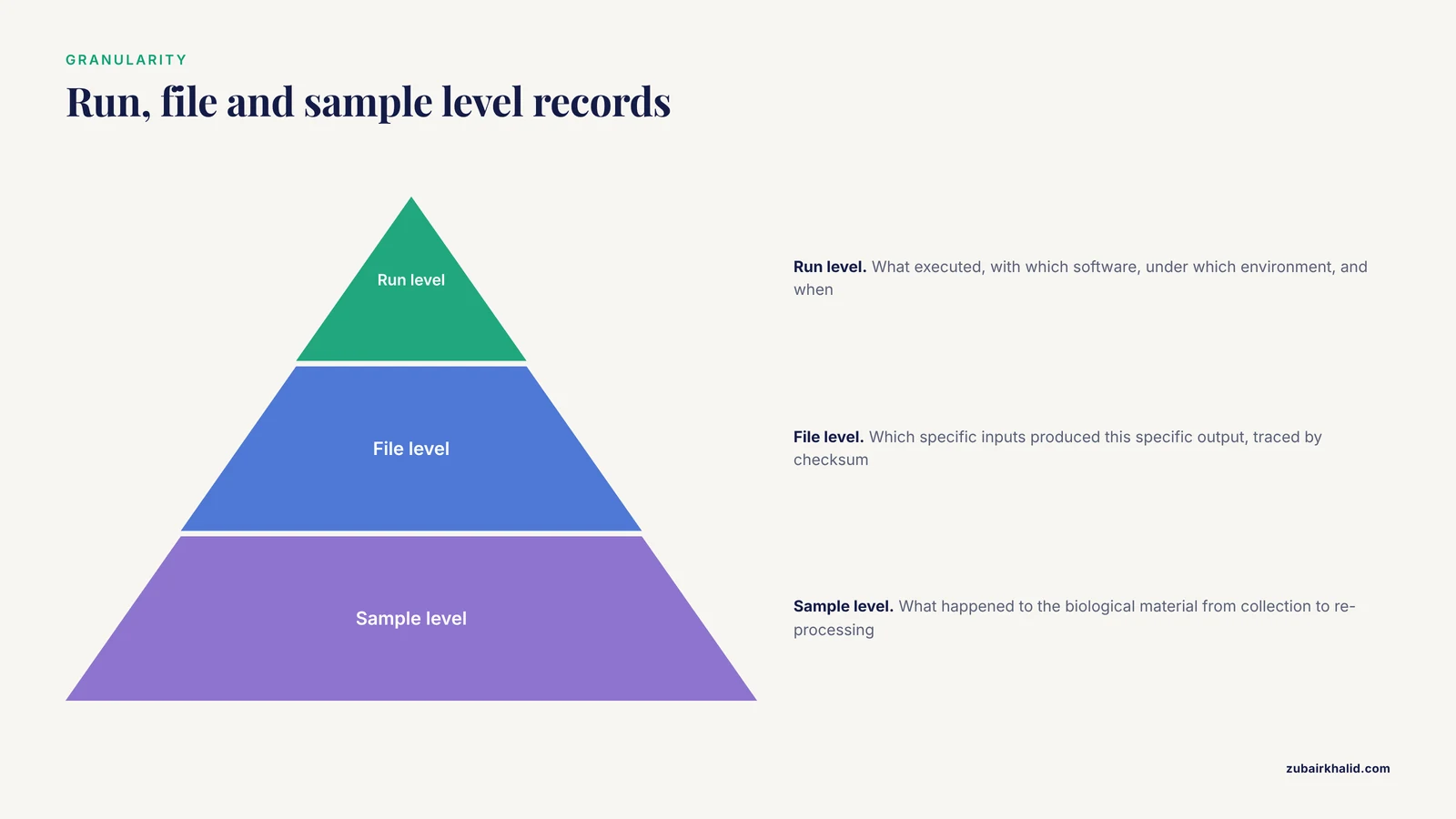
Provenance can be recorded at different granularities, and choosing the right level for each question prevents both under-recording and record bloat.
Run-level provenance answers: what executed, with what software, under what environment, and when. It is the level workflow engines capture natively, and it maps directly onto the execution and provenance domains of reporting standards [2]. Use run-level records for troubleshooting, for describing methods in a manuscript, and for demonstrating that a pipeline version was used consistently across a project.
File-level provenance answers: which specific inputs produced this specific output. It is the level at which checksums operate, and it is what lets you trace a single variant call back through an alignment to a sequencing run. File-level records are essential whenever outputs are redistributed independently of the run that made them, for example when a processed matrix is shared without the full pipeline.
Sample-level provenance answers: what happened to this biological material. Collection, extraction, library preparation, and re-processing events form a chain that no engine observes, because it spans bench work, instrument runs, and computational steps. This is the level the ISA data model addresses, capturing laboratory protocols and processes, and the ARC profile's contribution is aligning those assay-level records with workflow execution metadata in one coherent, queryable container [14].
The three levels are complementary, and the failure modes differ. Relying only on run-level records leaves you unable to trace an individual file. Relying only on file-level records loses the execution context. Relying only on sample-level records leaves the computation opaque. The single-cell field illustrates the cost of the gap: the MAMS standards exist because feature-observation matrices circulated without fields describing the software and workflows that produced them, forcing consumers to treat computational history as unknown [15].
A useful granularity heuristic: record automatically at the level your tooling observes, and record deliberately at the level your tooling cannot. The engine observes run and file levels; the laboratory must supply sample level. When a standard asks you to declare a granularity, such as the multiple granularity levels Workflow Run RO-Crate supports, match the declaration to how the record will be consumed: cohort assembly needs sample level, debugging needs run level, and file redistribution needs file level [11].
Standard Selection in Practice: A Decision Table
With several standards available, teams often stall on selection. The decision depends on who consumes the record and what they must do with it.
| Your consumer and goal | Best-fit standard | Why |
|---|---|---|
| - | - | - |
| A collaborator who must re-run the analysis | CWLProv or Workflow Run RO-Crate | These bundle workflow, graph, inputs, and outputs into a re-executable package [10][11] |
| A regulator or clinical reviewer who must audit the method | BioCompute Object | Domain-structured reporting built for communication among scientists, regulators, test developers, and clinicians [2] |
| A repository or consortium ingesting your data | Whatever the ingest specifies, commonly metadata plus checksums | Ingest-side validation enforces provenance quality at submission [3] |
| A downstream analyst integrating assays | Provenance-based identifiers or a shared crate profile | Cross-assay integration depends on lineage-aware IDs [17] |
| A wet-lab and computational joint audit | ISA-Workflow Run RO-Crate profile | Bridges laboratory process records with execution records [14] |
| Versioned dataset distribution | DVC-based packaging | Dataset-as-repository with managed versions and updates [16] |
Two selection cautions. First, the standards are not mutually exclusive. A CWLProv crate can sit inside a project whose reporting to a clinical collaborator takes BioCompute form, because both rest on the same underlying PROV graph model [5]. Second, do not let selection delay capture. A laboratory recording seven classes of information in plain files today is better positioned than one waiting for the perfect standard, because the fields map forward into any of the formats above. The BioCompute ecosystem's growth of tooling across platforms, including support in widely used cloud platforms, lowers the cost of adopting the reporting format when the time comes [12].
Misconceptions That Persist
"Provenance is a feature you buy by installing a tool." Tooling enables capture, but the record is only as complete as the fields nobody thought to record. The documented case of workflows that failed re-execution despite documentation shows that even well-intentioned capture misses implicit environment assumptions unless someone hunts for them [1].
"If it ran once, it will run again." Re-executability is an property of the record plus the environment, not of the code. Containers reduce environmental variance, but defaults, seeds, and reference versions still live outside the image, and each one is a divergence vector.
"Checksums are overkill for small projects." Checksums cost seconds and catch wrong-version files and silent corruption that filenames cannot. Small projects are precisely where a swapped file goes unnoticed, because nobody else is watching.
"The repository stores my provenance for me." A repository stores what you submit. Provenance quality is enforced at ingest in well-run archives, but the burden of producing the fields remains with the submitter [3]. A submission missing sample context is stored faithfully and remains unusable for context-dependent questions [4].
"Provenance guarantees correctness." A complete record lets a reviewer verify how a result was made; it does not force the result to be right. A pipeline with a wrongly specified reference produces beautifully documented wrong calls. Records support judgment, they do not replace domain expertise.
"Provenance is only for big consortia." The consortium examples, ENCODE's tens of thousands of experiments [3] and TCGA's petabyte corpus [7], show the ceiling of the practice, not its entry point. The entry point is a checksum and a manifest, which scale down to a single analysis on a laptop. The learning health system literature points to bioinformatics as the model precisely because the field built these habits early [6].
"Capturing provenance will slow the pipeline down." The per-run cost of writing logs, checksums, and manifests is negligible against the compute cost of genomics workloads. The real cost is organizational: deciding schemas, training staff, and reviewing records. Front-loading that cost is what prevents the far larger cost of an unreproducible result discovered at review time.
Team Practices: Handoffs, Reviews, and Onboarding
Provenance is a team sport, and most capture failures are coordination failures. Three practices make the record durable across personnel changes.
Handoff packets. When a project moves between analysts, laboratories, or institutions, the handoff should include the code repository with its history, the parameters committed beside the code, checksums for all retained data, the sample sheet, and the manifests for every retained run. A handoff missing any of these transfers a puzzle rather than a project. The three-system case study is, in effect, a handoff failure at scale: each system's implicit assumptions were exactly the things a receiving team would have to rediscover [1].
Provenance review in code review. When a pipeline change is proposed, review the provenance implications alongside the code: does the change alter a default that must now be recorded explicitly, does it introduce a new input whose checksum policy needs defining, does it change output naming that downstream records depend on? Treating provenance impact as a review dimension costs minutes per change and prevents the slow accumulation of unrecorded behavior.
Onboarding exercises built on real records. The fastest way to teach a new analyst the laboratory's provenance discipline is to have them re-execute a past analysis from its record alone, on a clean machine, and log every point where they needed to ask a question. Each question marks a gap in the record. This exercise doubles as a periodic audit and converts the lab's documentation from abstract policy into a concrete, tested artifact.
Agree on agent conventions. Records that name agents inconsistently, sometimes a person, sometimes a pipeline, sometimes an institutional group, defeat graph queries that aggregate responsibility. Decide whether automated runs are attributed to the pipeline, the person who triggered it, or both, and apply the convention uniformly. This matters most in clinical-adjacent settings, where the BioCompute framework's agent and error structures exist precisely so responsibility and failure handling can be stated unambiguously [2].
Auditing Your Own Records: A Quarterly Checklist
Provenance capture degrades quietly: a new tool gets added without a version pin, a sample sheet column stops being filled, a checksum step is skipped during a deadline crunch. A short periodic audit keeps the system honest.
Work through these checks once a quarter, or at the close of each major project phase:
- Pick three recent runs at random and attempt the re-execution test on a clean machine or a fresh container. Record every point where you needed information the record did not contain [10].
- Verify checksums for all outputs of the sampled runs against the recorded digests. Any mismatch means a results file changed after the run, and the cause needs investigating before the results are trusted.
- Open the last ten sample sheet rows and confirm every controlled-vocabulary field contains a legal value and every notes field is filled for anomalous samples. Contextual completeness is what surveillance and clinical reuse depend on [4].
- Grep the manifests for mutable container tags. Any digest-free reference is a repeatability defect to fix at the source.
- Confirm reference records include accession, version, and checksum, and that derived indexes point to the checksummed FASTA they were built from, closing the flat-file versioning gap that filenames alone cannot [8].
- Check that every retained results file has a record in the same storage tier, and that no results file has outlived its record or vice versa [7].
- Run one graph query end to end: from a final output, walk the PROV graph back to the original inputs and confirm every hop has an agent and a timestamp. A graph with an anonymous hop is a graph with a gap.
- Review the failure log from prior audits and confirm this quarter's sampled runs no longer exhibit last quarter's root causes.
The audit's output is not a pass or fail but a list of capture gaps, each of which becomes a one-line change to a template, a wrapper, or a checklist. Teams that audit quarterly converge on records that pass re-execution on the first attempt, which is the practical definition of provenance capture working.
Cost and Overhead Considerations
Teams resist provenance programs because they imagine large costs. Separating real from imagined costs makes the investment case honest.
Compute overhead is small. Writing logs, computing SHA-256 checksums, and serializing PROV graphs add a trivial fraction of runtime for workloads dominated by alignment, assembly, or statistical modeling. Checksumming multi-terabyte files is the one operation with noticeable cost, and it can be scheduled during transfer or generation rather than as a separate pass.
Storage overhead is modest but nonzero. Logs, manifests, and graphs are small relative to sequence data. The main storage decision is retention policy: keeping every intermediate file from every run is expensive, and unnecessary. Keep the record and the final outputs; allow intermediates to be regenerated from inputs under recorded parameters. This is the philosophy behind re-executable packages, which bundle what is needed to reproduce rather than every intermediate byte [10].
Human cost is the dominant term, and it is front-loaded. Designing the sample sheet schema, choosing the standards, training the team, and running the first audits consume real person-weeks. But these are one-time investments amortized across every subsequent project. The recurring cost after adoption is minutes per run.
The counterfactual cost is what justifies the program. An unreproducible analysis discovered at review or audit triggers repeated re-execution attempts, forensic reconstruction from shell history, and in the worst case re-sequencing or re-analysis of samples whose processing was never recorded. Provenance capture converts that tail risk into a small, predictable operating cost. The consortium experience shows the economics at scale: keeping tens of thousands of experiments interoperable through uniform, provenance-capturing pipelines is what makes the catalog usable by outside resources at all [3], and versioned, metadata-coupled archival is what keeps a petabyte corpus navigable [7]. At laboratory scale the same arithmetic holds with smaller numbers on both sides.
A pragmatic budgeting statement for a research group: expect the heaviest investment in the first quarter of adoption, a light recurring cost thereafter, and returns measured in avoided re-execution failures, faster manuscript preparation, and reviews that no longer stall on questions the record already answers.
Frequently Asked Questions
What is provenance capture in bioinformatics?
It is the automatic recording of the inputs, software versions, parameters, and execution conditions behind each data product, in a machine-readable form. The goal is that any output can be traced to its origins and re-created.
Is provenance the same as metadata?
No. Metadata describes what a dataset is, such as tissue and platform. Provenance records how it was made, linking files, tools, settings, and agents in a history graph.
Which provenance standard should I adopt?
Match the standard to the goal. Use CWLProv or Workflow Run RO-Crate for re-executable workflow runs, BioCompute Objects for standardized reporting to regulators or collaborators, and W3C PROV as the graph model underneath both.
Does my workflow engine already record everything?
No. Engines capture step-level lineage well, but you still need to pin container digests, reference versions, and sample context yourself, and commit parameters to version control.
How do I record provenance for data downloaded from public repositories?
Store the accession, the exact version or release, the download date, a checksum of the downloaded files, and the script or command used to fetch them.
How much detail is enough?
Enough that a stranger can re-execute the analysis on a clean machine and reproduce the outputs, verified by checksums. If a missing detail would change the result, record it.
Sources
- Investigating reproducibility and tracking provenance - A genomic workflow case study.
- Enabling precision medicine via standard communication of HTS provenance, analysis, and results.
- The ENCODE Uniform Analysis Pipelines.
- The Mpox contextual data specification package: a data curation toolkit to support collaborative pathogen genomic surveillance.
- Relating simulation studies by provenance-Developing a family of Wnt signaling models.
- Embedding data provenance into the Learning Health System to facilitate reproducible research.
- TCGA Expedition: A Data Acquisition and Management System for TCGA Data.
- Genome assemblies and annotations are not static and need support for tracking their evolution.
- FAIRly big: A framework for computationally reproducible processing of large-scale data.
- Sharing interoperable workflow provenance: A review of best practices and their practical application in CWLProv.
- Recording provenance of workflow runs with RO-Crate.
- Bioinformatics tools developed to support BioCompute Objects.
- Modeling and integration of N-glycan biomarkers in a comprehensive biomarker data model.
- Fusion of computational and experimental provenance in RO-Crate.
- Matrix and analysis metadata standards (MAMS) to facilitate harmonization and reproducibility of single-cell data.
- BioBricks.ai: a versioned data registry for life sciences data assets.
- Analysis of clinical, single cell, and spatial data from the Human Tumor Atlas Network (HTAN) with massively distributed cloud-based queries.