Protein Bioinformatics Project Ideas for Beginners
By Dr. Zubair Khalid, DVM, MS, PhD ·
By the end of this guide you will have finished a complete protein bioinformatics project on your own laptop. You will fetch a real protein sequence from UniProt, compute its physicochemical profile in Python, find its evolutionary relatives with BLAST, align them, build a protein interaction network from the STRING database, rank the hub proteins in Cytoscape, and package the whole thing into a written report using a reusable template. No wet lab, no server, and no budget are required. Every database and program mentioned here is free.
Before you start, have the following on hand:
- A computer with at least 8 GB of RAM and about 10 GB of free disk space
- Python 3.10 or newer, with the Biopython and requests packages installed
- R 4.2 or newer (you will add Bioconductor packages during the fourth walkthrough)
- A spreadsheet program such as Excel, LibreOffice Calc, or Google Sheets
- Roughly one evening per walkthrough
Protein bioinformatics is the use of computational methods to study proteins: their sequences, their structures, their interactions, and their abundance across conditions. The project ideas below are ordered from pure sequence work to network and structure work, and each one mirrors the design of published research so that what you build as a beginner has a real scientific shape.
What Protein Bioinformatics Actually Covers
Four layers make up the field, and the projects in this guide touch all of them.
- Sequence. What is the chain of amino acids? Sequences are stored in FASTA format, a plain-text format where a header line starts with the greater-than symbol and every following line carries single-letter amino acid codes.
- Structure. How does that chain fold? Structures come from the Protein Data Bank (PDB) and from predicted models in the AlphaFold database.
- Function and networks. What does the protein do and what does it talk to? Functional annotation uses the Gene Ontology (GO), a controlled vocabulary of biological process, cellular component, and molecular function terms, and KEGG, the Kyoto Encyclopedia of Genes and Genomes, which maps proteins onto signaling and metabolic pathways. Protein-protein interaction (PPI) networks treat proteins as nodes and their interactions as edges.
- Abundance. How much of the protein is present? Proteomics measures this with mass spectrometry, and studies report differentially expressed proteins (DEPs) between conditions the way gene studies report differentially expressed genes (DEGs).
The Published Blueprint Behind Every Project Idea
Almost every disease-focused bioinformatics paper follows the same skeleton: download public data, find molecules that differ between conditions, test which functions those molecules share, build an interaction network, nominate hub molecules, and validate the top candidates. Once you can see that skeleton, ten different projects become variations of one skill set.
Recent papers show the pattern clearly. An osteoporosis study pulled DEGs from the Gene Expression Omnibus (GEO) and GeneCards, ran GO, KEGG, and gene set enrichment analysis (GSEA), built a PPI network, and nominated eight hub genes for laboratory follow-up [1]. A Parkinson disease study layered weighted gene co-expression network analysis (WGCNA) on top, then used STRING, Cytoscape, the DAVID enrichment platform, the CytoHubba plugin, ROC curves, and finally molecular docking [2]. A polycystic ovary syndrome study added machine learning feature selection, a nomogram, and CIBERSORT immune deconvolution [3]. On the proteomics side, a serum study used data-independent acquisition (DIA) mass spectrometry, GO and KEGG enrichment, and experimental validation in cells and mice [4]. A neuroscience paper intersected two gene sets to find crosstalk genes, picked a hub, screened a candidate drug, and validated it in a mouse model [5]. Even a study protocol in a neighboring field shows the same architecture, pairing a literature meta-analysis with interaction prediction and pathway analysis [6]. The takeaway is direct: if you can run the walkthroughs in this article, you can execute the core of a publishable analysis pipeline.
Ten Protein Bioinformatics Project Ideas for Beginners
The table summarizes the ten projects, then each subsection explains what you do, where the data comes from, and what you finish with.
| # | Project | Core question | Main tools | Difficulty |
|---|---|---|---|---|
| 1 | Protein ID card | What are this protein's basic properties? | UniProt, ProtParam | 1 of 3 |
| 2 | Homolog hunt | Which proteins resemble mine, and where? | BLAST, MUSCLE | 1 of 3 |
| 3 | Family census | How many family members does an organism carry? | InterPro, Pfam, HMMER | 1 of 3 |
| 4 | Biomarker dossier | What is the evidence for one protein in one disease? | UniProt, TIMER, PubMed | 2 of 3 |
| 5 | DEGs to hub genes | Which genes change, and which sit at the network center? | GEO, limma, STRING, Cytoscape | 2 of 3 |
| 6 | Co-expression modules | Which gene modules track a trait? | WGCNA | 2 of 3 |
| 7 | Crosstalk analysis | What do two biological processes share? | Venn logic, STRING, Cytoscape | 2 of 3 |
| 8 | Proteomics reanalysis | Which proteins differ between patient groups? | PRIDE data, enrichment tools | 2 to 3 of 3 |
| 9 | Immune context | How does immune infiltration relate to my protein? | CIBERSORT, TIMER | 2 to 3 of 3 |
| 10 | Docking screen | Does a compound fit my hub protein? | AutoDock Vina, PyMOL | 3 of 3 |
Project 1: Build a Protein ID Card
Pick any protein and produce a one-page profile: length, molecular weight, isoelectric point, hydropathy, amino acid composition, and annotated features such as signal peptides or transmembrane regions. UniProt supplies the sequence and annotation, and ProtParam supplies the numbers. This is the fastest way to learn FASTA handling and REST APIs, and Walkthrough 1 below is a ready-made example you can finish in about an hour.
Project 2: Find Evolutionary Cousins With BLAST and an Alignment
Ask which proteins in other species resemble your protein and which residues are conserved. Run a BLAST search, download the top homologs (evolutionarily related proteins), align them with MUSCLE or Clustal Omega, and highlight identical columns. The deliverable is a hit table plus an alignment figure. A good stretch goal is adding a distant relative, such as a yeast or plant ortholog, and finding the residues that survive a billion years of divergence.
Project 3: Count a Protein Family Across a Genome
Genome papers routinely catalog how many members a protein family has in one organism, because family expansions hint at adaptation. The Astragalus mongholicus genome paper, for example, identified 33 genes encoding glutathione S-transferase enzymes and 23 genes for flavonoid biosynthesis enzymes, including UDP-glucosyltransferases [7]. Your beginner version: choose a family, such as protein kinases or zinc-finger proteins, scan one proteome with HMMER against Pfam models, and report the count and domain architecture of each member.
Project 4: Write a Single-Protein Biomarker Dossier
Choose one medically interesting protein and assemble every line of computational evidence about it. CD147, also called Basigin, a highly glycosylated single-pass transmembrane glycoprotein, is a model case: a published meta-analysis pooled 522 breast cancer tumors and 492 normal tissues, found higher CD147 expression in tumors, linked it to stage, grade, and lymph node metastasis, and used the TIMER database to connect it with immune cell infiltration [8]. Your dossier needs the same sections: expression, prognosis, function, and immune context, each with a figure or table.
Project 5: From Differentially Expressed Genes to Hub Proteins
Download a disease-versus-control dataset from GEO, call DEGs with limma, map them onto STRING, and rank hub genes (the most connected nodes) with CytoHubba. This is the exact pipeline of the osteoporosis study that produced eight hub genes, CDK1, CCNB1, TOP2A, FEN1, CDC6, FOXM1, CDC25A, and MCM2, linking cellular senescence to bone disease [1], and of the Parkinson study that started from 659 disease DEGs and 2,555 circadian-rhythm genes before nominating SNCA and DRD2 as connector proteins [2]. Walkthrough 4 implements it step by step.
Project 6: Detect Co-Expression Modules With WGCNA
WGCNA groups genes into modules whose members rise and fall together, then correlates each module with a trait such as disease severity. Published work used WGCNA to filter key module genes in the Parkinson analysis [2] and to intersect signals between polycystic ovary syndrome and atherosclerosis [3]. Your deliverable is a module-trait correlation heatmap plus a network drawing of the most connected module.
Project 7: Find Crosstalk Between Two Biological Processes
Take two gene or protein sets, for example endoplasmic reticulum stress and pyroptosis, intersect them, and ask which shared molecules act as bridges. The published version of this project found 13 crosstalk genes, identified NFE2L2 as the hub through Cytoscape, screened tert-butylhydroquinone as a candidate activating compound, and confirmed the mechanism experimentally in mice [5]. A beginner can reproduce the computational half in an afternoon using the Walkthrough 3 skills.
Project 8: Reanalyze a Public Proteomics Dataset
Proteomics asks which proteins change in abundance, and DIA (data-independent acquisition) is a mass spectrometry strategy that measures fragments systematically across samples. One published DIA study compared serum from primary aldosteronism patients with and without abdominal aortic calcification, found 38 differentially expressed proteins, 6 upregulated and 32 downregulated, ran GO and KEGG enrichment, and validated Tenascin-X in vascular smooth muscle cells and in mice [4]. Start gently: take a published supplementary protein table, run the enrichment analysis yourself, and compare your figures with the paper before attempting raw mass spectrometry files from the PRIDE archive.
Project 9: Connect a Protein to Immune Infiltration
Tumors and atherosclerotic plaques contain mixtures of immune cells, and tools such as CIBERSORT estimate those cell fractions from bulk expression data. The PCOS-atherosclerosis study used CIBERSORT, found abnormal immune infiltration, and tied it to six hub genes, CD163, LAPTM5, TNFSF13B, MS4A4A, FGR, and IRF1 [3], while the CD147 analysis used the TIMER database for the same purpose in breast cancer [8]. Your deliverable is a heatmap of estimated immune cell types correlated with your protein of interest.
Project 10: Dock a Compound Into a Hub Protein
Molecular docking predicts how a small molecule fits into a protein binding site. Published pipelines use docking as the final computational filter: the Parkinson study verified binding activity between candidate compounds and their protein targets [2], and the NFE2L2 study screened tBHQ computationally before confirming it at the bench [5]. Install AutoDock Vina, prepare a protein structure from the PDB or AlphaFold database, dock a ligand, and inspect the pose in PyMOL. Treat scores as rankings, not measured affinities.
The Starter Toolkit
Every tool below is free, and the web versions need no installation.
| Tool | Job it does | Access point |
|---|---|---|
| UniProt | Curated protein sequences and annotations | uniprot.org |
| NCBI BLAST | Similarity search against sequence databases | blast.ncbi.nlm.nih.gov or BLAST+ command line |
| ExPASy ProtParam | Physicochemical protein profiles | ExPASy web server |
| EMBL-EBI services | Clustal Omega alignments and Simple Phylogeny trees | ebi.ac.uk Tools portal |
| MUSCLE | Fast multiple sequence alignment | Command line |
| STRING | Interaction networks with confidence scores | string-db.org |
| Cytoscape | Network visualization, analysis, and hub ranking | cytoscape.org |
| GEO | Public gene expression data | NCBI GEO |
| PRIDE | Public proteomics data | EMBL-EBI |
| RCSB PDB and AlphaFold DB | Experimental and predicted structures | rcsb.org, alphafold.ebi.ac.uk |
| Bioconductor | limma, clusterProfiler, GEOquery in R | Bioconductor |
| PyMOL | Molecular graphics (free for individuals via open-source builds) | Command line or GUI |
Walkthrough 1: Turn a Protein Name Into a Quantitative ID Card
This walkthrough is a complete worked example for Project 1 using human p53, the tumor suppressor encoded by the TP53 gene.
Step 1. Install the Python packages.
python -m pip install biopython requestsStep 2. Fetch the sequence from UniProt. P04637 is the accession, the stable identifier, for human p53.
curl https://rest.uniprot.org/uniprotkb/P04637.fasta -o p53.fasta
head -2 p53.fasta
Expected output:
>sp|P04637|P53_HUMAN Cellular tumor antigen p53 OS=Homo sapiens OX=9606 GN=TP53 PE=1 SV=1
MEEPQSDPSIEPPLSQETFSDLWKLLPENNVLSPLPSQAMDDLMLSPDDIEQWFTEDPG
Step 3. Verify your installation with a toy sequence. Use a 20-residue sequence containing each amino acid once, so you can check your setup against hand calculations. Two formulas matter here. Molecular weight equals the sum of the average residue masses plus one water molecule (18.015 Da) for the termini. GRAVY, the grand average of hydropathy, equals the sum of Kyte-Doolittle hydropathy values divided by the residue count.
from Bio.SeqUtils.ProtParam import ProteinAnalysis

toy = ProteinAnalysis("ACDEFGHIKLMNPQRSTVWY")
print(round(toy.molecular_weight(), 1))
print(round(toy.isoelectric_point(), 1))
print(round(toy.gravy(), 2))
print(round(toy.aromaticity(), 2))
Expected output (rounded, small floating-point tails are normal):
2395.7
6.8
-0.49
0.15
You can confirm two of these by hand. The hydropathy values for the twenty letters sum to -9.8, and -9.8 divided by 20 gives the GRAVY of -0.49. Aromaticity is the fraction of phenylalanine, tryptophan, and tyrosine, which is 3 out of 20, or 0.15.
Step 4. Run the same analysis on p53.
lines = open("p53.fasta").read().splitlines()
seq = "".join(line for line in lines if not line.startswith(">"))
p53 = ProteinAnalysis(seq)
print(len(seq))
print(round(p53.molecular_weight(), 1))
Expected output: a length of 393 and a molecular weight close to 43,700 Da. Check yourself: the UniProt entry page lists the length and exact mass, and your numbers should match them closely. A nice teaching point hides here, because p53 earned its name from an apparent mass of about 53 kDa on gels even though the calculated mass is lower.
Step 5. Fill in the ID card. Record length, molecular weight, isoelectric point (the pH at which net charge is zero), GRAVY, aromaticity, and the UniProt annotation lines for domains, signal peptides, and transmembrane regions. Next steps: add the instability index and secondary structure fraction from the same class, then build cards for three proteins in one pathway and compare them side by side.
Walkthrough 2: Homolog Hunting With BLAST and an Alignment
Step 1. Install the command-line tools.
conda install -c bioconda blast muscleStep 2. Search a curated database. The E-value is the number of alignments at least this good that you would expect by chance when searching a database of that size, so smaller means stronger evidence, and 1e-5 is a conventional working cutoff for homolog detection.
blastp -query p53.fasta -db swissprot -remote -evalue 1e-5 -max_target_seqs 25 -outfmt "6 qseqid sseqid pident length evalue bitscore" -out p53_hits.tsv
head -5 p53_hits.tsv
Expected output shape (exact rows depend on the current database build):
P04637  sp|P04637|P53_HUMAN  100.000  393  ...
P04637  sp|...               ...      ...  ...
The columns are query id, subject id, percent identity, alignment length, E-value, and bitscore. The -evalue flag sets the significance cutoff, -max_target_seqs limits how many hits are kept, and -outfmt 6 produces machine-readable tabular output.
Step 3. Pull the top homologs and align them. Copy the FASTA files of the top five hits from UniProt into one file called homologs.faa, then:
muscle -in homologs.faa -out homologs.aln.faaThe output alignment gives every sequence the same padded length, with dashes marking gaps.
Step 4. Check the result. Three checks catch most problems. Your own protein should be the top hit at 100 percent identity. True homologs should sit several orders of magnitude below the 1e-5 cutoff. The alignment should span most of the protein, not one short patch.
Step 5. Sensible next steps. Build a phylogenetic tree with the EMBL-EBI Simple Phylogeny service, compute a percent identity matrix, and mark the residues that are identical across all species on your ID card from Walkthrough 1.
Walkthrough 3: Build and Mine a Protein Interaction Network
Step 1. Choose a protein set. For a demonstration, use the p53 pathway: TP53, CDKN1A, MDM2, BAX, and ATM.
Step 2. Download the network from the STRING API. Species 9606 is the NCBI taxonomy identifier for human.
import requests

params = {
    "identifiers": "TP53\rCDKN1A\rMDM2\rBAX\rATM",
    "species": "9606",
}
response = requests.get("https://string-db.org/api/tsv/network", params=params, timeout=60)
response.raise_for_status()
with open("p53_network.tsv", "wb") as handle:
    handle.write(response.content)
print(response.text.splitlines())
print(len(response.text.splitlines()) - 1, "interactions")
Expected output:
node1_string_id	node2_string_id	node1_name	node2_name	combined_score
10 interactions
Step 3. Understand the score. The combined score runs from 0 to 1, where higher means stronger supporting evidence. STRING documents confidence bands at 0.400 for medium confidence, 0.700 for high confidence, and 0.900 for highest confidence, and the 0.400 band is the website default. Keep only strong edges:
import csv

with open("p53_network.tsv") as handle:
    rows = list(csv.DictReader(handle, delimiter="\t"))
strong = [r for r in rows if float(r["combined_score"]) >= 0.7]
print(len(strong), "high-confidence interactions")
Step 4. Analyze in Cytoscape. Open Cytoscape, use File, then Import, then Network from File, and load p53_network.tsv. Run Analyze Network to get degree and betweenness for every node. Then install the cytoHubba app from the App Manager and rank nodes with the MCC (maximal clique centrality) method, which is the same ranking step used in published hub-gene pipelines [2].
Step 5. Check the result. All five input proteins should appear as nodes, and you should see a strong edge between TP53 and MDM2, one of the best-characterized interactions in the p53 pathway. Next steps: color nodes by score, export a figure for your report, and rerun the whole procedure on the DEG list from Walkthrough 4.
Walkthrough 4: From Public Expression Data to Hub Proteins
Step 1. Find a dataset on GEO. Search GEO for a disease of interest with the phrases "expression profiling by array" or "expression profiling by high throughput sequencing", pick a dataset with both disease and control groups, and download the expression matrix.
Step 2. Install the R packages.
install.packages("BiocManager")
BiocManager::install(c("GEOquery", "limma", "clusterProfiler", "org.Hs.eg.db"))
Step 3. Call the DEGs with limma. Replace GSEXXXXX with your chosen accession. The matrix should have genes as rows and samples as columns.
library(GEOquery)
library(limma)

gset <- getGEO("GSEXXXXX", GSEMatrix = TRUE)[[6]]
expression <- exprs(gset)
condition <- factor(c("control", "control", "case", "case"),
                    levels = c("control", "case"))
design <- model.matrix(~ condition)
fit <- eBayes(lmFit(expression, design))
results <- topTable(fit, coef = "conditioncase", number = Inf)
significant <- subset(results, adj.P.Val < 0.05 & abs(logFC) > 1)
write.csv(significant, "degs.csv")
Each parameter matters. The coef argument selects the case-versus-control coefficient that model.matrix created. adj.P.Val is the Benjamini-Hochberg adjusted p-value, which corrects for testing thousands of genes at once, and 0.05 with an absolute log2 fold change above 1 is a conventional starting threshold. logFC is the base-2 log of the fold change between groups.
Step 4. Map the significant genes onto STRING using the same API call pattern from Walkthrough 3, submitting your gene symbols in batches if the list is long, then import the result into Cytoscape and rank hubs with cytoHubba.
Step 5. Run enrichment with clusterProfiler.
library(clusterProfiler)
library(org.Hs.eg.db)

ego <- enrichGO(gene = rownames(significant), keyType = "SYMBOL",
                OrgDb = org.Hs.eg.db, ont = "BP", pAdjustMethod = "BH")
head(as.data.frame(ego))
The ont argument selects the biological process branch of GO, and pAdjustMethod = "BH" applies the same multiple-testing correction as limma.
Step 6. Check the result. Plot a volcano map of logFC against adjusted p-value and confirm the significant count is plausible for the dataset, usually tens to a few thousand genes. Confirm that the top GO terms relate to the disease biology rather than to ribosome or housekeeping artifacts. Confirm your hub genes actually appear in the network you imported. Then validate the shortlist in an independent dataset, which is the step published pipelines perform through external validation sets [3]. This walkthrough is the beginner-scale version of the published GEO-to-network pipelines described in Projects 5 and 6.
A Reusable Write-Up Format and Template
Every project above becomes a portfolio piece if you write it up in a consistent format. The same skeleton works for a blog post, a GitHub README, and eventually the methods section of a manuscript. Copy this template into your notes for each project:
1. Question (one sentence)
2. Data (database, accession numbers, download date)
3. Methods (every tool with its version and every parameter you set)
4. Results (figures and tables, numbered)
5. Checks (what you verified and how)
6. Limitations (what could make the result wrong)
7. Next steps (the one experiment or analysis you would run next)
A filled example for Project 1 reads as follows. Question: what are the physical properties of human p53? Data: UniProt P04637, downloaded on the date of analysis. Methods: UniProt REST, Biopython ProtParam, default parameters. Results: 393 residues, calculated mass near 43,700 Da, hydrophilic profile, annotated DNA-binding domain. Checks: mass and length match the UniProt entry. Limitations: calculated properties ignore post-translational modifications. Next steps: compare with p53 orthologs from Walkthrough 2. If your larger goal is to learn bioinformatics as a discipline, treat each finished template as one chapter of your education, and pair the sequence with a structured bioinformatics course for the statistics and graph theory underneath, since a course explains why limma moderates variance and why centrality measures disagree, while these projects give that theory something real to land on.
Common Errors and Exact Fixes
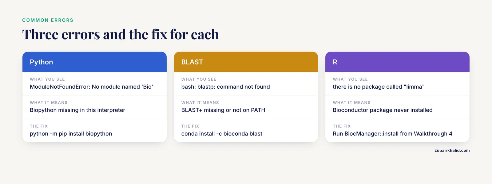
ModuleNotFoundError: No module named 'Bio'means Biopython is not installed in the interpreter you are running. Fix withpython -m pip install biopython, or useconda install -c conda-forge biopythonif you manage environments with conda.bash: blastp: command not foundmeans BLAST+ is missing or not on your PATH. Install withconda install -c bioconda blastand open a fresh terminal.ValueError: More than one record found in handlecomes from Biopython when you useSeqIO.readon a multi-record FASTA file. Switch toSeqIO.parseand loop over the records.- An HTTP 404 from rest.uniprot.org means the accession does not exist in that form. Search the protein name on uniprot.org and copy the exact accession.
Error in library(limma) : there is no package called "limma"means the Bioconductor package was never installed. Run theBiocManager::installcommand from Walkthrough 4.java.lang.OutOfMemoryError: Java heap spaceappears in Cytoscape when a network is too large for the default memory allocation. Raise the Java heap setting in the Cytoscape launch configuration as described in the Cytoscape user manual, or import a filtered network with high-confidence edges only.requests.exceptions.ConnectionErroragainst the STRING API is usually a network problem or brief server maintenance. Retry with thetimeoutargument set, and check that your identifiers use official symbols.- BLAST returning no hits at all usually means the query file contains a header with no sequence beneath it, or the sequence contains stop characters. Print the file, confirm real residues follow the header, and loosen the expect threshold if the protein is very short.
Common Mistakes and Limitations
Beginners tend to make the same handful of mistakes, and each has a direct fix.
Treating predicted interactions as proven physical bindings is the most common error. STRING aggregates several kinds of evidence, including text mining, so an edge means supporting evidence exists, not that two proteins were co-crystallized. Filter by score and read the evidence legend.
Confusing statistical significance with biological importance comes second. An adjusted p-value says an difference is unlikely under the null hypothesis, not that it is large or useful, which is why the fold-change cutoff exists alongside it.
Skipping the multiple-testing correction invalidates a DEG list entirely. Testing 20,000 genes at the raw 0.05 level guarantees thousands of false positives, so always report adjusted values.
Ignoring batch effects ruins cross-dataset conclusions. Before any differential analysis, plot the samples with principal component analysis and confirm that samples separate by biology rather than by processing date or platform.
Reading centrality as causality is subtle but widespread. A hub gene is a hypothesis generator, and the published pipelines treat it that way, following computation with experiments in cells or animal models [5] [4].
Overtrusting docking scores rounds out the list. Docking ranks compounds, it does not measure affinity, and every docking-led study cited here moved to experimental confirmation before making claims [5].
Finally, keep reproducibility. Record tool versions, parameters, and download dates in the template, because a result you cannot rerun is not a result. And one boundary statement belongs here: none of these projects produces a clinical claim, computational output is a hypothesis for laboratory follow-up, and individual health decisions belong with a qualified clinician.
Frequently Asked Questions
Do I need to know how to program before starting these projects?
No, but you need the willingness to copy and modify short scripts. Projects 1 through 4 can be done almost entirely with web tools, and the two command-line walkthroughs here use fewer than fifteen lines of code each, which is enough to learn from.
Which protein bioinformatics project should a beginner do first?
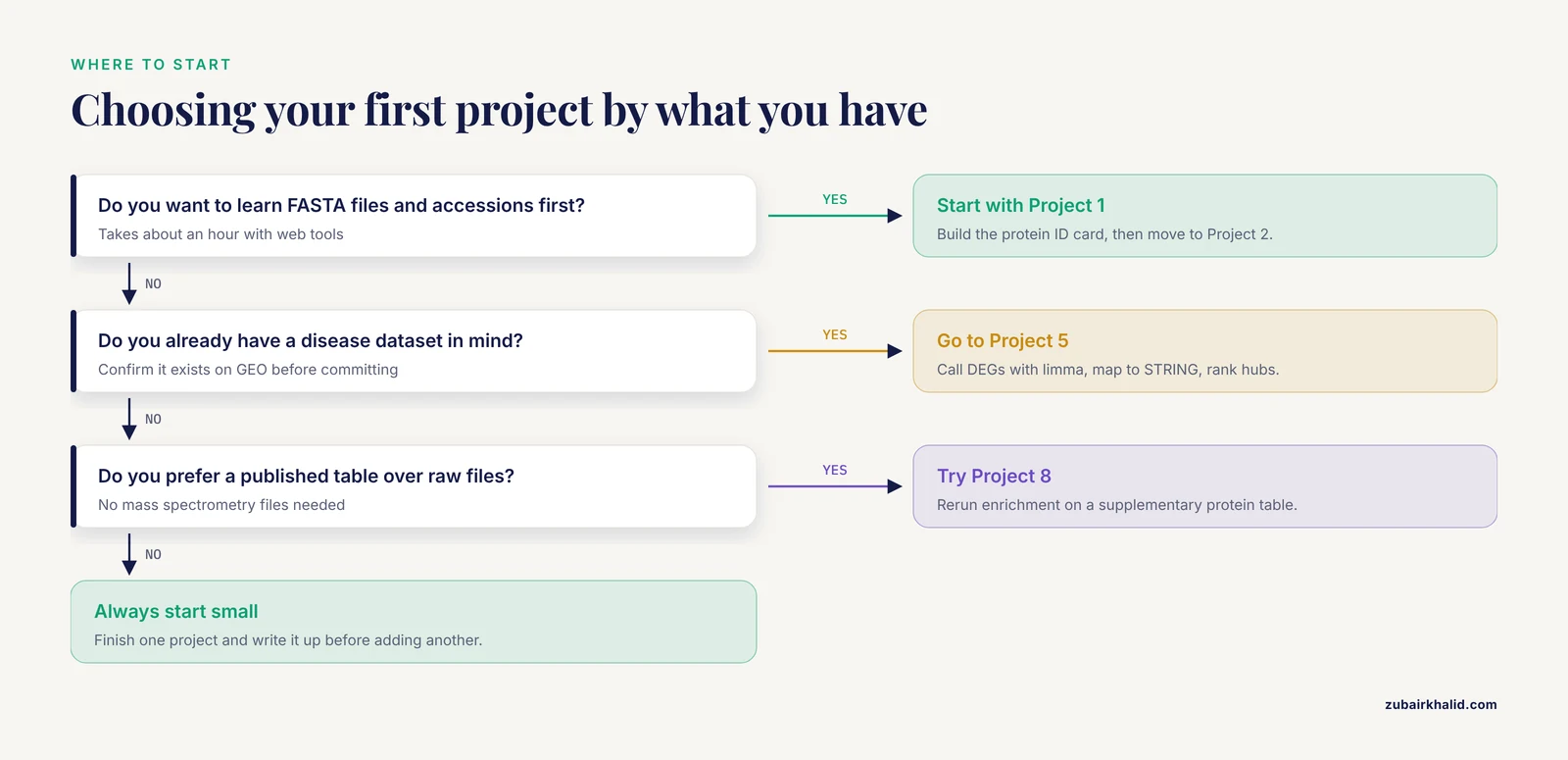
Start with Project 1, the protein ID card, because it teaches FASTA files, accessions, and property calculations in about an hour. Move to Project 2 next, since BLAST and alignment skills support every later project.
Can I complete these projects with free tools only?
Yes. UniProt, NCBI, EMBL-EBI services, STRING, Cytoscape, GEO, PRIDE, and academic licenses for PyMOL are all free, and none of the walkthroughs in this guide requires paid software or cloud spending.
How do I pick a protein or disease for my project?
Pick something you already care about, then confirm data exists by searching GEO or UniProt before committing. A protein with rich annotation and a disease with several public datasets will keep every project stage moving.
How long does a beginner protein bioinformatics project take?
Plan on one evening for Projects 1 through 3, one to two weekends for Projects 4 through 7, and several weeks for the proteomics, immune, and docking projects. The write-up template adds an hour but saves days when you revisit the work.
Can a beginner project turn into something publishable?
A beginner project alone rarely clears the publication bar, but it can become the pilot analysis for one. The published studies described here are essentially the same pipelines executed with more datasets, stricter validation, and laboratory confirmation, so a well-documented beginner project is a legitimate first draft of those sections.
How is protein bioinformatics different from genomics or transcriptomics?
Genomics studies DNA sequence and variation, transcriptomics studies RNA abundance, and protein bioinformatics focuses on the molecules that actually execute most cellular functions. In practice they interlock, since DEG lists from transcriptomics are routinely mapped onto protein networks.
What should I learn after finishing these projects?
Learn statistics for high-throughput data, then bulk RNA-seq pipelines, then single-cell methods, adding one Python or R skill with each project. Repeating Project 5 on a new disease with your own parameter choices is the cleanest bridge to independent work.
Sources
- Integrated Bioinformatics Analysis and Experimental Validation of the Role of Cellular Senescence in Osteoporosis.
- Identification of SNCA and DRD2 as key genes linking parkinson's disease and circadian rhythm through bioinformatics analysis.
- Identification of crucial genes for polycystic ovary syndrome and atherosclerosis through comprehensive bioinformatics analysis and machine learning.
- Inverse association between the extracellular matrix protein Tenascin-X and concurrent abdominal aortic calcification in patients with primary aldosteronism.
- Activation of NFE2L2 Alleviates Endoplasmic Reticulum Stress-Mediated Pyroptosis in Murine Hippocampus: A Bioinformatics Analysis and Experimental Validation.
- Long noncoding RNA as a biomarker for the prognosis of ischemic stroke: A protocol for meta-analysis and bioinformatics analysis.
- The whole-genome map of Astragalus mongholicus provides ideas for the synthesis of glutathione and flavonoid.
- CD147 expression as a clinicopathological and prognostic indicator in breast cancer: a meta-analysis and bioinformatics analysis.