How to Plot Protein Domains in Python
By Dr. Zubair Khalid, DVM, MS, PhD ·

By the end of this guide you will be able to fetch a protein sequence and its domain annotations, turn those annotations into clean coordinate data, and render both a single-protein domain diagram and a multi-protein comparison figure using Python for bioinformatics. You will also know how to validate the result, which errors to expect, and where the common mistakes are. The workflow uses Python 3.10 or later, Biopython, matplotlib, and public annotation databases (UniProt, Pfam, and InterPro), and everything runs on a standard laptop with an internet connection.
Python has become the default language for biological visualization. Phylogenetic tools such as the ETE Toolkit anchor a whole ecosystem of Python packages for annotating and rendering large trees [1], and even beamline operations in structural biology now run on Python-based client-server visualization stacks [2]. Domain diagrams are a natural part of that ecosystem: once you can draw residue-level intervals, the same pattern extends to heatmaps, networks, and phylogenetic overlays.
Prerequisites and Environment Setup
Install the libraries you need with pip:
python -m pip install biopython matplotlib requests pyhmmerWhat each package does:
| Package | Role in this workflow |
|---|---|
| , - | , - |
| biopython | Sequence I/O, NCBI Entrez access, UniProt XML parsing |
| matplotlib | Static rendering of domain diagrams |
| requests | Optional, cleaner HTTP calls than urllib |
| pyhmmer | Python bindings for HMMER, for running Pfam scans locally |
You also need the domain annotations themselves. A protein domain is a conserved, independently folded or functionally recognized segment of a protein sequence. Domains are annotated by expert-curated databases: Pfam, which is part of InterPro at EMBL-EBI, defines domains as profile hidden Markov models (HMMs) matched to protein families. UniProt combines automatic and manual annotations, including domains, regions, motifs, repeats, and sites. InterPro integrates member databases such as Pfam, SMART, and PROSITE under one interface.
You should be familiar with two coordinate conventions before writing any plotting code:
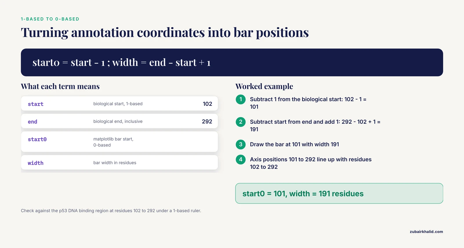
- Biological annotation databases use 1-based, inclusive coordinates. Residue 102 through 292 inclusive means a segment 191 residues long.
- matplotlib uses 0-based coordinates and draws bars as (start, width) pairs, which are half-open intervals on the axis.
Almost every off-by-one error in domain plots comes from mixing these two conventions. The conversion rule you will use repeatedly is: matplotlib start equals biological start minus 1, and matplotlib width equals biological end minus biological start plus 1. For residues 102 to 292, that gives a bar starting at 101 with width 191, covering axis positions 101 through 292, which visually lines up with residues 102 through 292 under a 1-based ruler.
Where Protein Domain Data Comes From
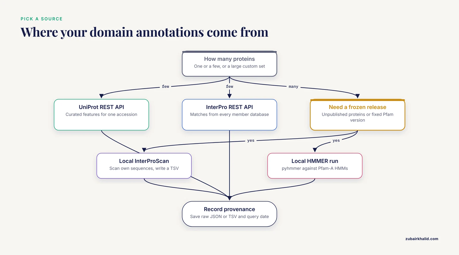
You have three practical sources for domain annotations, and the choice affects reproducibility:
- UniProt REST API. Query one accession and receive JSON with curated features. Best for small sets of proteins and for features beyond domains, such as active sites and disordered regions.
- InterPro REST API. Query one protein and receive matches from every InterPro member database, including Pfam, with precise per-database coordinates.
- Local InterProScan or HMMER runs. Scan your own sequences against Pfam-A HMMs and produce a tab-separated file. Best for large custom datasets, unpublished proteins, or versions you want frozen.
Annotations change between database releases. If you query live APIs, record the accession, the API URL, and the query date with your figure, or save the raw JSON response next to your script. This habit matters because scripted, parameterized workflows are replacing manual inspection across bioinformatics [3], and a figure you cannot regenerate is a figure you cannot defend.
How to Plot Protein Domains in Python, Step by Step
This walkthrough plots the canonical human p53 protein (UniProt accession P04637, 393 residues) end to end. The same script works for any accession.
Step 1: Fetch and Verify the Sequence
from Bio import SeqIO
import urllib.request

accession = "P04637"
fasta_url = f"https://rest.uniprot.org/uniprotkb/{accession}.fasta"
urllib.request.urlretrieve(fasta_url, f"{accession}.fasta")

record = SeqIO.read(f"{accession}.fasta", "fasta")
print(record.id, len(record.seq))
Expected output:
sp|P04637|P53_HUMAN 393This is the classic Biopython tutorial pattern: read a FASTA file into a SeqRecord, then use len(record.seq) to get the protein length. Keep the length variable handy because it sets the x-axis limit for your figure.
Step 2: Fetch Domain Annotations as JSON
import json
import urllib.request

url = f"https://rest.uniprot.org/uniprotkb/{accession}.json"
with urllib.request.urlopen(url) as response:
    data = json.load(response)

protein_length = data["sequence"]["length"]
print("Length:", protein_length)
print("Number of features:", len(data.get("features", [])))
Each feature in the features list has a type (for example Domain, Region, Site, DNA binding), a description, and a location with numeric start.value and end.value fields, 1-based inclusive. Extract the ones you want to plot:
DOMAIN_TYPES = ("Domain", "Region", "Family", "Repeat",
                "Coiled coil", "DNA binding", "Zinc finger")

domains = []
for feat in data.get("features", []):
    if feat["type"] in DOMAIN_TYPES:
        loc = feat["location"]
        start = loc["start"].get("value")
        end = loc["end"].get("value")
        if start is None or end is None:
            continue  # unresolved boundaries, cannot plot
        domains.append({
            "name": feat.get("description") or feat["type"],
            "type": feat["type"],
            "start": start,
            "end": end,
        })

for d in sorted(domains, key=lambda x: x["start"]):
    print(f'{d["start"]:>4} {d["end"]:>4} {d["type"]:<12} {d["name"]}')
Expected output shape (values are typical for the canonical human p53 sequence, but re-query before you publish because annotation releases update coordinates):
 102  292 DNA binding   DNA binding
 102  292 Domain        p53
 325  355 Region        Tetramerization
 367  386 Region        Regulatory
Always print this table before plotting. If the numbers look wrong here, the figure will be wrong too, and a coordinate table is much easier to debug than a rendered diagram.
Step 3: Build a Reusable Drawing Function
The workhorse matplotlib call is Axes.broken_barh, which accepts a list of (start, width) tuples and a (bottom, height) pair. Write the drawing as a function so you can reuse it for single proteins and stacked comparisons:
import matplotlib.pyplot as plt
import matplotlib as mpl

def draw_protein(ax, domains, protein_length, y=0.0, height=0.6,
                 color="#4C72B0", show_labels=True, fontsize=8):
    for d in domains:
        start0 = d["start"] - 1                 # 1-based to 0-based
        width = d["end"] - d["start"] + 1       # inclusive to half-open
        ax.broken_barh([(start0, width)], (y, height),
                       facecolors=d.get("color", color),
                       edgecolor="black", linewidth=0.8)
        if show_labels:
            ax.text(start0 + width / 2, y + height / 2, d["name"],
                    ha="center", va="center", fontsize=fontsize)
    ax.set_xlim(0, protein_length)
    ax.set_yticks([])

fig, ax = plt.subplots(figsize=(10, 1.8))
draw_protein(ax, domains, protein_length)
ax.set_xlabel("Residue position")
ax.set_title("Human p53 (P04637), UniProt annotations")
fig.savefig("p53_domains.svg", bbox_inches="tight")
plt.show()
The result is a single horizontal bar 393 residue units long with colored boxes over the annotated segments, each labeled with its name. The saved SVG is vector graphics, which means journals and slides can scale it without pixelation.
Key parameters in broken_barh:
| Task | Function or parameter | Notes |
|---|---|---|
| , - | , - | , - |
| Draw one or more domain bars | ax.broken_barh(xranges, yrange) | xranges is a list of (start, width) tuples in 0-based coordinates |
| Stagger overlapping domains | second element of yrange, the vertical offset | Use small lane offsets like 0.0, 0.8, 1.6 |
| Outline each domain | edgecolor="black", linewidth=0.8 | Thin outlines keep adjacent domains visually distinct |
| Label inside the bar | ax.text(x_center, y_center, label) | ha="center", va="center" centers the text |
| Set the axis to protein length | ax.set_xlim(0, protein_length) | Without this, the plot auto-scales and looks misleading |
| Add a residue ruler | ax.set_xticks(range(0, length + 1, 50)) | Ticks every 50 or 100 residues read well |
| Export for publication | fig.savefig("figure.svg") | Use dpi=300 or higher for PNG and TIFF |
| Flip protein order top to bottom | ax.invert_yaxis() | Keeps the first row of your input list at the top |
Step 4: Plot Several Proteins in One Figure
Comparative domain diagrams are where this approach pays off. Build a list of proteins by fetching each accession, assign a consistent color per domain name across all rows, and stack the rows:
import matplotlib as mpl
import matplotlib.pyplot as plt
import urllib.request, json

def fetch_protein(accession):
    url = f"https://rest.uniprot.org/uniprotkb/{accession}.json"
    with urllib.request.urlopen(url) as response:
        data = json.load(response)
    desc = data["proteinDescription"]["recommendedName"]["fullName"]["value"]
    domains = []
    for feat in data.get("features", []):
        if feat["type"] in ("Domain", "Region"):
            s = feat["location"]["start"].get("value")
            e = feat["location"]["end"].get("value")
            if s is not None and e is not None:
                domains.append({"name": feat.get("description") or feat["type"],
                                "start": s, "end": e})
    return {"id": accession, "name": f"{desc} ({accession})",
            "length": data["sequence"]["length"], "domains": domains}

proteins = [fetch_protein(acc) for acc in ("P04637", "P02340")]  # human, mouse p53

fig, ax = plt.subplots(figsize=(11, 1 + 0.8 * len(proteins)))
cmap = mpl.colormaps["tab20"]
domain_colors = {}
max_len = max(p["length"] for p in proteins)

for row, p in enumerate(reversed(proteins)):
    for d in p["domains"]:
        if d["name"] not in domain_colors:
            domain_colors[d["name"]] = cmap(len(domain_colors) % 20)
        d["color"] = domain_colors[d["name"]]
    draw_protein(ax, p["domains"], p["length"], y=row, height=0.6,
                 color="lightgray", show_labels=False)

ax.set_yticks([r + 0.3 for r in range(len(proteins))])
ax.set_yticklabels([p["name"] for p in reversed(proteins)])
ax.set_xlabel("Residue position")
ax.set_xlim(0, max_len)
ax.invert_yaxis()

handles = [plt.Rectangle((0, 0), 1, 1, facecolor=c) for c in domain_colors.values()]
ax.legend(handles, domain_colors.keys(), loc="upper center",
          bbox_to_anchor=(0.5, -0.25), ncol=3, fontsize=8)
fig.savefig("p53_orthologs_domains.svg", bbox_inches="tight")
The figure shows one row per protein with shared colors for shared domain names, so conserved architecture is visible at a glance. This is the step-by-step core of how to plot protein domains in Python for real comparative work.
Step 5: Handle Overlapping Annotations With Lanes
Different databases often annotate overlapping or nested segments on the same protein, for example a Domain inside a broader Region. Drawing them all at the same y-offset stacks them invisibly. Assign lanes greedily:
def assign_lanes(domains):
    lane_ends = []
    for d in sorted(domains, key=lambda x: x["start"]):
        placed = False
        for i, last_end in enumerate(lane_ends):
            if d["start"] > last_end:      # 1-based inclusive: no overlap
                d["lane"] = i
                lane_ends[i] = d["end"]
                placed = True
                break
        if not placed:
            d["lane"] = len(lane_ends)
            lane_ends.append(d["end"])
    return domains

domains = assign_lanes(domains)

fig, ax = plt.subplots(figsize=(10, 1 + 0.8 * (max(d["lane"] for d in domains) + 1)))
for d in domains:
    start0 = d["start"] - 1
    width = d["end"] - d["start"] + 1
    ax.broken_barh([(start0, width)], (d["lane"], 0.6),
                   facecolors="#4C72B0", edgecolor="black")
    ax.text(start0 + width / 2, d["lane"] + 0.3, d["name"],
            ha="center", va="center", fontsize=8)
ax.set_xlim(0, protein_length)
ax.set_yticks([])
Each overlapping annotation now sits on its own horizontal lane, and you can color by source database if you mix UniProt and Pfam matches.
Step 6: Scale the Figure to the Sequence
A 3,000-residue protein needs a wider canvas than a 150-residue domain. Set the figure width proportional to length and bump the font only if it stays readable:
width_inches = max(6, protein_length / 60)
fig, ax = plt.subplots(figsize=(width_inches, 2))
This keeps residue positions comparable across figures of different proteins, which matters when you paste several diagrams into one document.
Working With Pfam and InterProScan Output
When you need Pfam domains for many sequences, or for proteins not in UniProt, run InterProScan or HMMER locally and plot from the tabular output. InterProScan writes a TSV file where the columns you care about are: protein accession, sequence length, analysis name, signature accession, signature description, start, stop, score, status, date, InterPro accession, and InterPro description.
import csv

def parse_interproscan_tsv(path):
    records = {}
    with open(path) as handle:
        for line in handle:
            if line.startswith("#"):
                continue
            f = line.rstrip("\n").split("\t")
            protein_id = f
            length = int(f[4])
            hit = {
                "name": f[5] or f[6],     # description, fallback to accession
                "analysis": f[1],
                "start": int(f[7]),
                "end": int(f[8]),
            }
            records.setdefault(protein_id, {"length": length, "domains": []})
            records[protein_id]["domains"].append(hit)
    return records

all_proteins = parse_interproscan_tsv("interproscan.tsv")

fig, ax = plt.subplots(figsize=(12, 1 + 0.8 * len(all_proteins)))
for row, (pid, rec) in enumerate(reversed(list(all_proteins.items()))):
    draw_protein(ax, rec["domains"], rec["length"], y=row,
                 color="#55A868", show_labels=False)
    ax.text(-0.02 * rec["length"], row + 0.3, pid,
            ha="right", va="center", fontsize=9)

ax.set_xlim(0, max(r["length"] for r in all_proteins.values()))
ax.set_yticks([])
ax.set_xlabel("Residue position")
If you want to scan directly from Python rather than shelling out to hmmscan, pyhmmer provides Python bindings to the HMMER engine, and its documentation includes quickstart examples for scanning sequences against an HMM file such as Pfam-A. You will need the compressed Pfam-A HMM database downloaded locally, which is several hundred megabytes.
One caution on scores: Pfam matches carry profile scores and gathering thresholds, and neither belongs on the spatial axis of a domain diagram. A domain bar should occupy its residue interval, full stop. If you want to display match quality, encode it as bar opacity or as a separate column of summary plots, not as bar length. The same discipline applies to domain-motif interaction data: when researchers plot binding intensities for the full human PDZ domain set against peptide motifs, they keep the quantitative values in dedicated charts rather than distorting domain geometry [6].
Customization Tips for Publication-Quality Figures
These plot protein domains python tips separate a quick draft from a figure you can publish:
- Use one palette per domain name, globally. Build the color map once, as in Step 4, so the same domain is the same color in every panel of a multi-panel figure.
- Distinguish annotation sources. UniProt curated domains, Pfam matches, and predicted regions deserve different visual treatments, such as solid fill versus hatching or dashed outlines. If a figure mixes sources silently, readers will assume they are equivalent evidence.
- Annotate sites on top of domains. Active sites, phosphorylation sites, and mutation hotspots are point features. Draw them as vertical markers with
ax.plot(x, y, marker="^")or thinaxvlinecalls at the residue position minus 1. - Show low-complexity and disordered regions as background. A light gray background span from residue a to b tells the reader why there are no domain bars there, which is information, not empty space.
- Save both SVG and PNG. Vector output for the manuscript, 300 dpi raster for quick sharing.
bbox_inches="tight"prevents label clipping. - Freeze your inputs. Save the JSON or TSV you plotted from, plus the query date. If a reviewer asks how a domain coordinate was obtained, you can answer exactly.
- Number labels when they collide. For short proteins crowded with small domains, put the domain index inside the bar and expand the index to the name in the legend.
For interactivity, plotly renders the same coordinate data as hoverable shapes:
import plotly.graph_objects as go

fig = go.Figure()
for d in domains:
    fig.add_shape(
        type="rect",
        x0=d["start"] - 1, x1=d["end"],
        y0=0, y1=1,
        fillcolor="#4C72B0", line=dict(color="black"),
    )
    fig.add_annotation(x=(d["start"] + d["end"]) / 2, y=0.5,
                       text=d["name"], showarrow=False, font=dict(size=10))
fig.update_xaxes(range=[0, protein_length], title="Residue position")
fig.update_yaxes(visible=False)
fig.show()
Hover text can carry the exact start, end, source database, and e-value for each domain, which is useful when you share figures with collaborators who need the numbers. For larger exploratory tools, bioinformatics teams increasingly wrap plotting code in small web apps, the pattern Streamlit-based visualization companions use in modern pipelines [3].
Checking Your Figure Is Right
Validate on three levels before trusting the rendering:
- Coordinate check. Sum the widths of non-overlapping domains and compare against the annotated intervals. A domain listed as 102 to 292 must render as a bar whose left edge sits at 101 on the 0-based axis and spans 191 units.
- Cross-reference check. Open the same protein on the UniProt or InterPro websites and compare your figure against their built-in viewers, which use the same underlying annotation records. Mismatches usually mean you filtered a different feature type or mixed isoform coordinates.
- Independence check. If you plotted from a local InterProScan run, verify one or two proteins against the live InterPro API for the same release. Scripted cross-checks are more reliable than eyeballing, a principle that motivated recent statistical tools replacing visual-inspection workflows in single-cell analysis [7].
Also confirm the sequence length in your FASTA matches the sequence.length field in the JSON. If they differ, you may have downloaded a different isoform, which changes every downstream coordinate.
Common Mistakes and Limitations
These are the errors that show up again and again when people first plot protein domains in Python:
- Off-by-one shifts. Passing UniProt start values straight into
broken_barhshifts every bar right by one residue. Always convert withstart - 1and compute width asend - start + 1. - Calling
plt.broken_barh. The function lives on the Axes object.plt.broken_barh(...)raisesAttributeError: module 'matplotlib.pyplot' has no attribute 'broken_barh'. Useax.broken_barh(...). - Unresolved feature boundaries. UniProt features such as some chain or region annotations can have
nullstart or end values when boundaries are not pinned to specific residues. Accessingfeat["location"]["start"]["value"]then raisesKeyError: 'value'. Filter those features out, as Step 2 does, or plot them as edge indicators with qualitative styling. - Isoform mixups. UniProt accessions map to a canonical sequence, but domain coordinates are isoform-specific. Plotting canonical coordinates onto a short isoform sequence produces bars that run past the protein end. Check the length field every time.
- Overlapping bars stacked silently. Without lane assignment, a nested domain hides the one beneath it. Use the
assign_lanesfunction from Step 5, or plot one database per figure. - Auto-scaled axes. If you forget
ax.set_xlim(0, protein_length), matplotlib scales to the drawn bars and a protein with one small domain looks like it is all domain. Set the limit explicitly. - Score-based misinterpretation. A Pfam match has a score and a gathering threshold. Reporting a low-scoring match as a solid, definitive domain bar overstates the evidence. Consider showing match quality as opacity, and when a match is marginal, say so in the caption.
- Label collisions in dense proteins. Text wider than its bar overlaps neighboring labels. Use indexed labels with a legend, shorten names to accessions, or rotate labels vertically.
- Hardcoded colors and names. A script with a hardcoded list of domains is not reproducible. Fetch the annotations, or at minimum load them from a saved file with a recorded provenance.
- Treating the diagram as structure. A domain map shows annotated sequence intervals, not three-dimensional folding, and not domain boundaries at residue resolution. Domain boundaries themselves are models with uncertainty between releases.
A related limitation concerns what happens after the diagram. Domain architecture is one input into protein function, but prioritizing candidates or interpreting disease relevance requires additional evidence layers such as expression, interaction networks, and enrichment analysis, which computational pipelines assemble from resources like GEO, UniProt, STRING, KEGG, and Gene Ontology [8]. Your figure is a starting point, not an endpoint.
Beyond Static Diagrams: Extending the Workflow
Once the coordinate-to-graphics pattern is in place, the same machinery extends in several directions that current Python bioinformatics actively supports:
- Variant effects along domains. Multiplexed assays of variant effects (MAVEs) produce residue-level scores that map naturally onto domain intervals. The sortscore Python package computes Sort-seq activity scores from binned counts and provides heatmap visualizations, demonstrated on deep mutational scanning data for the transcription factor GLI2 [9]. Overlaying such scores onto a domain diagram turns an architecture figure into a structure-function figure.
- Sequence-design evaluation. If you generate or redesign protein sequences computationally, libraries such as seqme provide model-agnostic metrics and visualization functions for evaluating designed proteins against target distributions [4]. Domain plots help you check whether designed variants preserve expected domain architecture.
- Evolutionary context. Placing domain diagrams beside a gene tree contextualizes duplications and losses. The ETE Toolkit ecosystem handles large phylogenies with rich annotation layers [1], and PhyloZoo provides a Python framework with dedicated visualization tools and robust input-output for phylogenetic networks, installable from PyPI [10].
- Interaction networks. Domain-mediated interactions can be drawn as networks with NetworkX, the approach used in multi-database protein interaction pipelines that integrate expression, annotation, and interaction resources [8].
- Large-scale exploratory analysis. For high-dimensional omics data with visualization needs beyond single proteins, unified Python frameworks such as PySimi support similarity construction, spectral clustering, and downstream visualization, and their evaluations show that method choices measurably change biological interpretation [5].
Frequently Asked Questions
Do I need Biopython to plot protein domains in Python?
No, Biopython is convenient but not required. A domain plot needs only three things per protein: a length, a list of intervals, and labels, all of which can come from a plain JSON or TSV file you parse with the standard library. Biopython earns its place when you also handle sequences, GenBank records, alignments, or structures, and its UniProt XML and FASTA readers save real time in those cases.
Which is better, UniProt annotations or running Pfam myself with HMMER?
For one or a few well-characterized proteins, use UniProt or the InterPro API, because the annotations are curated and stable to cite. For large custom datasets, unpublished sequences, or when you must freeze a specific Pfam release, run InterProScan or HMMER locally and plot from the TSV output. Many projects do both, live queries for well-annotated proteins and local scans for everything else.
Why are my domain bars shifted by one residue?
You passed 1-based inclusive coordinates directly into matplotlib, which expects 0-based (start, width) pairs. Convert with start0 = start - 1 and width = end - start + 1. Check a single well-known domain, such as the p53 DNA-binding region at residues 102 to 292, and confirm the bar spans exactly that interval under a 1-based residue ruler.
How do I plot domains from several proteins in one figure?
Fetch each protein into a list of dictionaries with length and domain intervals, draw one row per protein with broken_barh at increasing y offsets, set the x-axis to the maximum length, and share one color map keyed by domain name so orthologous domains match across rows. The loop in Step 4 of the walkthrough is a complete working template.
Can I plot intrinsically disordered regions and motifs the same way?
Yes. UniProt exposes disordered regions, motifs, compositional bias, and repeats as features with the same coordinate structure as domains, so the identical drawing function handles them. Use a different visual style, such as hatching or pale fill, and consider drawing them as background lanes beneath the domain bars so domain architecture remains the visual focus.
How do I make publication-quality domain diagrams?
Render with matplotlib to SVG or PDF, set the figure width proportional to sequence length, keep one global color per domain name, add a residue-position ruler with ticks every 50 to 100 residues, and save the annotation source and query date alongside the figure. If the diagram will appear beside structure figures, match font sizes and line weights to your other panels.
Can I make interactive domain plots?
Yes. Plotly draws the same intervals as hoverable rectangles, so each domain can carry its exact coordinates, source database, and match score in a tooltip. For shared exploratory tools, teams increasingly wrap plotting code in lightweight web applications, a pattern now common in modern bioinformatics pipelines with Streamlit-based visualization companions.
How do I cite Pfam or InterPro when I publish a domain figure?
Cite the database itself, not this workflow: name the database release or version you used, the accessions of the entries plotted, and the retrieval date for API queries. Pfam is a member database of InterPro at EMBL-EBI, and UniProt provides the merged feature annotations, so a figure built from UniProt features credits UniProt, while a figure built from InterProScan output against Pfam-A credits Pfam through InterPro.
Sources
- An Integrated Ecosystem for Analysis and Visualization of Large-Scale Phylogenomic Data Combining ETE Toolkit, TreeProfiler, and PhyloCloud for Scalable Phylogenomic Analysis.
- QuickProcess2: an integrated package for crystallography data visualization, processing and management at the GM/CA Structural Biology Facility.
- PerSeqPIPE: Nextflow workflow for per-sequence analysis of small RNA-sequencing data.
- seqme: a Python library for evaluating biological sequence design from generative models.
- PySimi: a unified framework for similarity measure evaluation in spectral clustering with applications to omics data.
- A Computational Protocol to Analyze PDZ/PBM Affinity Data Obtained by High-Throughput Holdup Assay.
- Quantifying distribution shifts in single-cell data with scXMatch.
- Computational prioritization of breast cancer biomarker candidates through automated protein-protein interaction network analysis: A multi-database framework.
- sortscore: Sort-seq MAVE scoring and visualization using Python.
- PhyloZoo: a unified framework for phylogenetic network analysis in Python.