How to Build a Phylogenetic Tree from Orthologous Genes in R
By Dr. Zubair Khalid, DVM, MS, PhD ·

By the end of this guide you will be able to take a set of protein or nucleotide sequences, confirm they are true orthologs, produce a cleaned multiple sequence alignment, select a substitution model, and build a bootstrap-supported maximum likelihood phylogenetic tree, all with commands you can copy into R today. This is a practical R for bioinformatics workflow, and the alignment, sequence handling, and visualization stages rely on Bioconductor packages, so it also works as a Bioconductor tutorial for phylogenetics.
Everything here assumes you have R 4.2 or later, RStudio or another IDE, and about 20 GB of free disk space if you plan to run orthology detection on whole genomes. The tree-building steps themselves run on a laptop in minutes for datasets up to a few hundred sequences.
Why Orthologous Genes Are the Right Input
An ortholog is a gene in two species that descended from a single gene in their last common ancestor, usually retaining the same function. A paralog is a copy created by duplication within a lineage. Mixing paralogs into your dataset is the single fastest way to build a tree that reflects gene duplication history rather than species relationships, so orthology verification comes before any alignment or tree inference.
Recent comparative genomics studies make the logic concrete. A phylogenomic analysis of firefly genera identified 1,011 nuclear single-copy orthologs using BUSCO and OrthoFinder and used them to resolve relationships that mitochondrial genomes alone could not settle [1]. A comparative study of the fungus Cadophora luteo-olivacea built a phylogenomic tree from 2,645 single-copy orthologs to place a divergent strain outside the main species clade [2]. A bacterial study of Streptococcus sinensis used a core single-copy ortholog phylogeny to show that the species sits closest to S. cristatus, followed by S. sanguinis and S. gordonii [3]. A chloroplast genome study of the endangered tree Madhuca pasquieri reconstructed relationships with 69 orthologous genes under maximum likelihood [4]. The common thread is single-copy orthologs, inferred with a reproducible tool, then aligned and analyzed gene by gene.
The field has converged on two design decisions you will face immediately. First, how to find the orthologs. Second, whether to build one tree per gene and reconcile them, or concatenate genes into one supermatrix. Both appear in current literature. The firefly study found discordance between concatenation-based and coalescence-based phylogenies, which pointed to incomplete lineage sorting, and used filtering for compositional homogeneity and clock-likeness to refine their marker panel [1]. Your workflow should preserve the ability to do both.
What You Need Before You Start
Install the following, in this order.
- R 4.2 or newer from CRAN.
- Bioconductor packages, installed with BiocManager. This covers the Bioconductor portion of the workflow.
- CRAN packages: ape, phangorn, seqinr, and ggtree support tools.
- Optional but recommended command-line tools: OrthoFinder for orthology detection across genomes, MAFFT for fast protein alignments, and IQ-TREE if you eventually outgrow phangorn.
The tree-building core, alignment coercion, and visualization all live in R, so you can prototype entirely inside R for small sequence sets and only reach for command-line tools when scaling to genome-scale ortholog detection.
Step-by-Step Workflow for a Phylogenetic Tree from Orthologous Genes in R
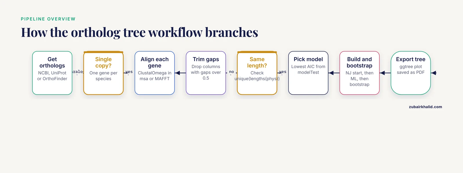
Step 1. Install and Load the R Packages
Open R and run:
install.packages("BiocManager")
BiocManager::install(c("msa", "Biostrings", "DECIPHER", "ggtree"))
install.packages(c("ape", "phangorn", "seqinr", "ggplot2"))
Then load them at the top of a fresh script:
library(BiocManager)
library(Biostrings)
library(msa)
library(DECIPHER)
library(ape)
library(phangorn)
library(seqinr)
library(ggtree)
library(ggplot2)
Confirm versions so your analysis is reproducible:
sessionInfo()Save the output of sessionInfo() alongside your results. Anyone reproducing your tree later will need to know that you used, for example, phangorn 2.11.1 and ape 5.7. Version drift in alignment and tree packages is a real reproducibility risk, not a theoretical one.
Step 2. Collect and Verify Orthologous Sequences
For a small set of species where you already know the gene of interest, download homologous protein sequences directly from NCBI GenBank or UniProt, save them as a FASTA file, and move to Step 3.
For genome-scale work, use OrthoFinder outside R. Place one FASTA file of predicted proteins per species in a folder, then run:
orthofinder -f ~/data/proteomes -t 16OrthoFinder assigns every gene to an orthogroup, writes per-orthogroup FASTA files, and produces a file listing single-copy orthogroups, which are orthogroups containing exactly one gene from every species. Those single-copy orthogroups are your candidate markers. This is the same combination of BUSCO completeness assessment and OrthoFinder orthology inference used to identify the 1,011 single-copy orthologs in the firefly phylogenomic study [1], and it mirrors the logic of combining multiple annotation methods, where no single tool recovers every ortholog [5].
In R, read one orthogroup into memory and sanity-check it:
seqs <- read.fasta("OG0000413.fa", seqtype = "AA", as.string = TRUE)
length(seqs)
sapply(seqs, length)
Expected output looks like this:
[6] 12
   Homo_sapiens    Mus_musculus   Gallus_gallus ...
             412            409             396 ...
Two checks matter here. Confirm that every species you expect is represented exactly once, and confirm that no sequence is suspiciously short, which usually means a fragment or a mispredicted gene model. Drop fragmented sequences now rather than after tree building. Quality control at this stage, including genome annotation quality measured by BUSCO, is what makes later ortholog sets trustworthy, as the tunicate comparative genomics study demonstrated when it restricted its phylogenetic analysis to species with gene models scoring above 80 percent BUSCO completeness [7].
Step 3. Build the Multiple Sequence Alignment
The msa package ships binaries for ClustalOmega, ClustalW, and MUSCLE, so no external installation is needed:
aa <- readAAStringSet("OG0000413.fa")
aln <- msa(aa, method = "ClustalOmega", order = "input")
aln
Expected output:
CLUSTAL multiple sequence alignment (ClustalOmega)

Homo_sapie...  MEEPQSDPSV---SGAGSAG...
Mus_muscu...   MEEPQSDPSIELP SQEFSAG...
Gallus_gal...  MEEPQSDLSG---NAGSAG...
Three parameters matter. method sets the aligner. ClustalOmega is a good default for proteins. order = "input" keeps sequence order stable between runs, which simplifies downstream bookkeeping. For nucleotide sequences, add type = "DNA" so msa knows the alphabet.
For large datasets, run MAFFT in a shell and bring the result back into R:
mafft --auto OG0000413.fa > OG0000413.aligned.faphys <- read.phyDat("OG0000413.aligned.fa", format = "fasta", type = "AA")The choice of aligner is not cosmetic. Alignment error propagates directly into tree error, and a recent evaluation of alignment cleaning found that removing likely alignment errors from alignments, and from the alignments used to train substitution models, measurably improved gene tree inference for single-copy orthologs [6]. Treat alignment quality as a first-class concern, not a checkbox.
Step 4. Inspect and Trim the Alignment
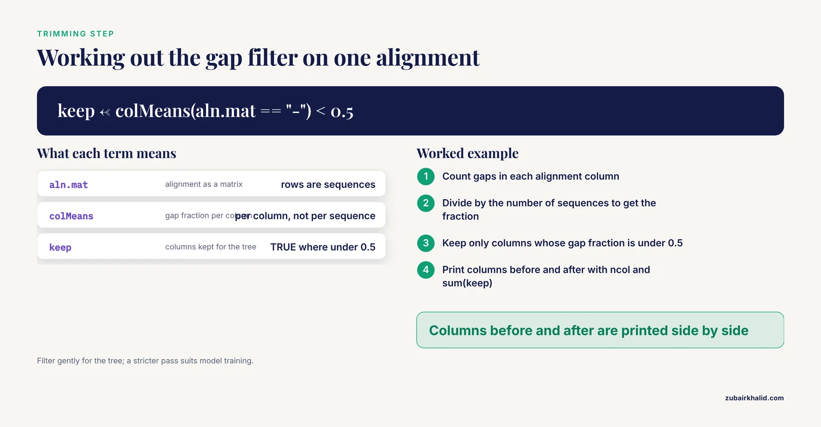
Raw alignments carry columns that are all gaps, or nearly all gaps, from poorly aligned or poorly conserved regions. These columns add noise. A transparent, scriptable filter is better than an opaque one:
aln.mat <- as.matrix(aln)
gap.fraction <- rowMeans(aln.mat == "-")  # per sequence, not per column
col.gaps <- colMeans(aln.mat == "-")
keep <- col.gaps < 0.5
aln.trimmed <- aln.mat[, keep]
cat("Columns before:", ncol(aln.mat), "\n")
cat("Columns after: ", sum(keep), "\n")
Write the trimmed alignment back out for downstream tools:
trimmed.seq <- apply(aln.trimmed, 1, paste, collapse = "")
write.fasta(sequences = as.list(trimmed.seq),
            names = rownames(aln.trimmed),
            file.out = "OG0000413.trimmed.fa")
Here is where a real evidence-based decision enters the workflow. Stringent filters, which cut aggressively, remove more error but also more genuine signal. A benchmark-driven comparison of filtering strategies found that stringent filtering produced the biggest gains when training substitution models, while gentle filtering of the per-gene alignments themselves gave the best gene tree inference, with the consensus-based CLOAK algorithm performing best overall because it removes likely errors with a low false positive rate [6]. In practical terms, filter gently for the alignment you tree from, and if you train or refit substitution models, consider a stricter pass.
Load the trimmed alignment for tree building:
phys <- read.phyDat("OG0000413.trimmed.fa", format = "fasta", type = "AA")Confirm all sequences are the same length, because this is the error that bites most often later:
unique(lengths(phys))If this prints one number, you are clean. If it prints several, an alignment step was skipped or a file was mixed up.
Step 5. Concatenate Multiple Genes or Keep Them Separate
With one gene, skip this step. With many single-copy orthologs, decide between a concatenated supermatrix and per-gene trees.
For concatenation, align each gene separately first, remove gappy columns per gene, then bind them:
gene.files <- list.files(pattern = "OG.*\\.trimmed\\.fa$")
phys.list <- lapply(gene.files, read.phyDat,
                    format = "fasta", type = "AA")
names(phys.list) <- tools::file_path_sans_ext(gene.files)
concatenated <- do.call(rbind.phyDat, phys.list)
If you get this error, the cause is almost always an unaligned or differently filtered gene file:
Error in rbind.phyDat(phys.list) : sequences are not all of the same lengthThe fix is to recheck each gene file in phys.list with unique(lengths()) before binding. Sequence lengths differ across genes, so binding requires the same taxa in the same order in every partition, not the same column count across genes. Ensure species names match exactly, including case and underscores, across all files.
Keep per-gene trees as well. The firefly study compared concatenation- and coalescence-based phylogenies and found discordance indicating incomplete lineage sorting, the failure of different genes in the same genome to share one genealogy because ancestral polymorphisms persisted through speciation [1]. A concatenated tree averages over that discordance, which is fine for some questions and misleading for others.
Step 6. Choose a Substitution Model
A substitution model describes the probabilities of one residue changing into another over evolutionary time, plus rates for transitions versus transversions and rate variation across sites. phangorn can test the standard set:
mt <- modelTest(phys, model = "all", G = TRUE, I = TRUE)
head(mt[order(mt$AIC), ], 8)
Expected output resembles:
      Model df    logLik      AIC      BIC
1        LG 46 -18432.21 36956.42 37168.55
2     LG+I 47 -18430.88 36955.76 37174.16
3    LG+G4 49 -18424.03 36946.06 37177.01
4  LG+I+G4 50 -18423.71 36947.42 37184.64
5       WAG 46 -18461.90 37015.80 37227.93
6    WAG+G4 49 -18449.15 36996.30 37227.25
Pick the model with the lowest AIC, the Akaike information criterion, which balances fit against model complexity. For protein alignments, LG and WAG dominate empirical model lists. For nucleotide data from coding regions, GTR plus gamma-distributed rate variation is the standard general-time-reversible choice.
The model matters beyond routine fitting. Wheeler and colleagues showed that substitution models trained on filtered alignments improve gene tree inference, with stricter filtering giving the largest model improvements [6]. In other words, model choice and alignment cleaning interact, so revisit the model after you finalize the trimming strategy rather than treating model selection as a one-time step.
Step 7. Build the Tree
Start with a distance-based neighbor-joining tree as a starting topology. Neighbor joining builds a tree greedily from a pairwise distance matrix, is fast, and provides a sensible starting point for maximum likelihood:
dm <- dist.ml(phys, model = "JTT")
tree_nj <- NJ(dm)
plot(tree_nj, cex = 0.7)
Then refine with maximum likelihood, which searches for the topology, branch lengths, and model parameters that maximize the probability of observing your alignment:
fit <- pml(tree_nj, data = phys, k = 4)
fit_opt <- optim.pml(fit, model = "LG", rearrangement = "stochastic",
                     control = pml.control(trace = 0))
fit_opt
Expected output:
loglikelihood: -18424.03

Rate matrix:  LG
...
Number of tips: 12
Two parameters deserve explanation. k = 4 sets four discrete rate categories to approximate gamma-distributed rate variation among sites. rearrangement = "stochastic" performs randomized tree rearrangements during the search, which reduces the chance of getting stuck on a local optimum at some cost in runtime. For nucleotide data, substitute model = "GTR" and dist.ml(phys, model = "raw") or the appropriate model-corrected distance.
If you see this error, your tip labels and sequence names do not match:
Error in pml(tree_nj, data = phys) : tree and data do not matchFix it by reconciling names:
common <- intersect(tree_nj$tip.label, names(phys))
phys <- subset(phys, taxa = common)
tree_nj <- drop.tip(tree_nj, setdiff(tree_nj$tip.label, common))
Root the tree with an outgroup, a taxon known to fall outside your group of interest, so that the direction of evolution is defined:
tree_rooted <- root(fit_opt$tree, outgroup = "Aureobasidium_pullulans",
                    resolve.root = TRUE)
Step 8. Assess Support with Bootstrap Resampling
A bootstrap analysis resamples alignment columns with replacement many times, rebuilds a tree from each resampled dataset, and reports how often each split in your tree is recovered. It answers how sensitive the topology is to which sites happened to be in the alignment, not whether the tree is true.
bs <- bootstrap.pml(fit_opt, bs = 100, trees = TRUE,
                    control = pml.control(trace = 0))
tree_bs <- plotBS(fit_opt$tree, bs, type = "phylogram")
For real analyses, raise bs to 500 or 1,000 and run it in parallel with multicore = TRUE if your system allows. Expect runtime to scale roughly linearly with the number of replicates and steeply with the number of taxa.
For per-gene trees destined for a coalescent species tree summary, export the replicate trees or the consensus per gene rather than bootstrapping the concatenation:
write.tree(bs[[6]], "OG0000413_bs1.tre")Step 9. Visualize and Export the Final Tree
ggtree, a Bioconductor package, turns the tree into a publication-grade plot:
p <- ggtree(tree_bs, size = 0.8) +
     geom_tiplab(size = 3, fontface = "italic") +
     geom_nodelab(aes(label = label), hjust = -0.15, size = 2.5,
                  color = "steelblue") +
     geom_treescale(x = 0, y = -0.2)
p
ggsave("ortholog_tree.pdf", p, width = 8, height = 6)
The blue node labels are bootstrap percentages. Tip labels inherit your FASTA headers, which is why clean, consistent sequence naming in Step 2 pays off here.
Reference Table of Key Options
| Decision | Options | Practical guidance |
|---|---|---|
| Orthology tool | OrthoFinder, BUSCO, BLAST reciprocal best hits | OrthoFinder plus BUSCO for genome-scale panels [1] |
| Aligner | ClustalOmega, MUSCLE, ClustalW (msa), MAFFT | ClustalOmega for proteins in R, MAFFT for large sets |
| Gap filter threshold | Column gap fraction under 0.3 to 0.7 | Filter gently for gene trees, more strictly when training models [6] |
| Substitution model, protein | LG, WAG, JTT, with +G and +I | Select by lowest AIC from modelTest |
| Substitution model, DNA | JC69, HKY, GTR, with +G and +I | GTR+G for most coding DNA |
| Tree method | Neighbor joining, maximum likelihood | NJ for a starting tree, ML for the final one |
| Bootstrap replicates | 100 (exploratory), 500 to 1,000 (final) | Higher is better when runtime allows |
| Multi-gene strategy | Concatenation, per-gene trees with coalescent summary | Report both when discordance is possible [1] |
Tips That Improve Tree Quality
- Use proteins for deep divergences. Amino acid alignments remain informative across hundreds of millions of years where nucleotide alignments saturate. Use DNA for closely related taxa where synonymous-site information helps.
- Verify single-copy status before trusting any gene. The bacterial S. sinensis study leaned on a core single-copy ortholog phylogeny precisely because single-copy status anchors orthology assumptions [3]. OrthoFinder's single-copy orthogroup list is the practical filter.
- Combine annotation sources when predicting genes from new genomes. A comparison of BRAKER2, BUSCO, Miniprot, and Scipio showed each tool recovered orthologs the others missed, and combining them produced a more complete ortholog dataset for swallowtail butterflies [5]. If your input genes come from your own annotation, run more than one predictor.
- Align each gene separately, always. Concatenating unaligned genes produces garbage that R will accept without complaint, which is worse than an error.
- Keep an outgroup from the start. Post hoc rerooting changes interpretation of ancestral character states and can change apparent topology when branch lengths are short.
- Record every parameter. The reproducibility of a tree from orthologous genes in R depends on versions, aligner settings, filtering thresholds, and the model, not just the sequence data.
- For large ortholog panels, evaluate marker quality per gene. The firefly study filtered single-copy orthologs for compositional homogeneity, clock-likeness, and species-tree concordance, which reduced 1,011 markers to 103 high-quality SCOs, and used that filtered panel for final inference [1]. Quality filtering of markers is standard practice in current phylogenomics, not an optional extra.
Common Mistakes and Limitations
Building the tree from paralogs. If a gene duplicated before your species diverged, each copy has its own history. Duplicated copies in an alignment make species appear artificially distant or cluster gene copies by function. Check single-copy status with OrthoFinder or a reciprocal best hit search, and remove or model duplicated lineages explicitly. The P-COGs framework was designed partly because multi-isoform handling and incomplete datasets break naive ortholog grouping, and it encourages one sequence dataset for both ortholog inference and tree construction [8].
Skipping alignment cleaning, or over-cleaning. Both extremes have documented costs. Removing alignment errors improves gene trees, but harsh filters also delete informative residues and can make trees worse, which is why the CLOAK consensus-based approach was built as a gentle filter with a low false-positive removal rate [6]. Match filter stringency to the downstream task.
Assuming pairwise distance equals phylogeny. Distance-based clustering without proper phylogenetic inference can produce groups that are not monophyletic on the actual tree. In tuberculosis transmission inference, pairwise SNP-distance clustering generated non-monophyletic clusters in an endemic setting even at a 25 SNP threshold, while showing strong phylogenetic consistency at higher thresholds in a low-transmission dataset [9]. If your downstream question depends on cluster membership, verify clusters against a tree.
Interpreting a concatenated tree as the species tree without checking for conflict. Incomplete lineage sorting and other gene-tree discordance mean concatenated and coalescent summaries can disagree, as the firefly phylogenomics showed [1]. When concatenation and coalescent trees disagree, report both and investigate the conflicting nodes rather than publishing whichever looks nicer.
Ignoring model selection. Running pml with the default JC69 or JTT and never testing alternatives wastes the information in your data. Run modelTest, and remember that alignment filtering changes which model fits best [6].
Over-trusting bootstrap values. A bootstrap percentage is a resampling statistic. High values mean the split is stable given your data and model. They do not certify correctness when the model is wrong, the alignment is biased, or taxon sampling is sparse.
Forgetting that this is one article's workflow, not a regulatory standard. For clinical microbiology questions, such as whether an isolate belongs to a transmission cluster, phylogenetic trees are one input among epidemiological and laboratory evidence, and the Thailand tuberculosis study demonstrates how settings change the behavior of the same methods [9].
Frequently Asked Questions
Can I build a phylogenetic tree from orthologous genes in R without command-line tools?
Yes, for small datasets. The msa package includes built-in ClustalOmega, MUSCLE, and ClustalW binaries, and ape plus phangorn handle model testing, tree building, and bootstrapping. Command-line tools become necessary mainly for genome-scale orthology detection.
How many orthologous genes do I need for a reliable tree?
More genes generally mean better resolution, and published panels range from 69 orthologous genes in a plant chloroplast study to 2,645 single-copy orthologs in a fungal phylogenomic analysis [4][2]. The right number depends on how closely related your taxa are and how much conflict among genes you expect.
What is the difference between a gene tree and a species tree?
A gene tree records the ancestry of one gene, which can differ from the species tree because of gene duplication, loss, or incomplete lineage sorting. Building per-gene trees and summarizing them under a coalescent model is the standard response when the two disagree.
Should I align DNA or protein sequences?
Align proteins when your taxa span deep evolutionary distances, because amino acids are more conserved and align more reliably. Align nucleotides, ideally codon-aware, for closely related species where synonymous substitutions carry signal.
What bootstrap value counts as strong support?
Bootstrap values above roughly 70 percent are conventionally treated as moderate to strong support for a split, and values above 90 percent as strong. Treat these as conventions, not laws, and always report the replicate count alongside the values.
How do I handle paralogs in my dataset?
Identify them with orthology tools or reciprocal best hits, then either exclude them, restrict analysis to one copy per species, or model duplication explicitly with a gene-tree reconciliation approach. Tools built for orthologous group discovery, such as P-COGs, help surface duplication events that naive pipelines miss [8].
Why are my bootstrap values low even with many genes?
Low support usually reflects a short internal branch, meaning a rapid radiation, conflicting signal among genes, or an inadequate model. Check per-gene concordance, revisit alignment filtering, and compare concatenation against coalescent summaries before concluding the data are inadequate.
Can I use this workflow for bacterial whole genomes?
Yes, with core single-copy orthologs across your isolate set, which is exactly the approach used to place Streptococcus sinensis within the viridans group streptococci [3]. For very closely related isolates, core genome SNP phylogenies are often used alongside ortholog-based trees [10].
Sources
- Nuclear single-copy orthologous genes as phylogenomic markers for resolving the closely related firefly genera Pteroptyx, Medeopteryx, and Trisinuata (Coleoptera: Lampyridae: Luciolinae).
- Comparative genomics of Cadophora luteo-olivacea reveals a divergent lineage, conserved functional repertoires, and strain-level phenotypic variation.
- Comparative genomics identifies a cyl-like region in Streptococcus sinensis isolates from a patient with infective endocarditis.
- Comparative analysis of morphology and chloroplast genomes in endangered plant Madhuca pasquieri and two congeneric plants: revealing phylogenetic relationships.
- Combining Annotation Software to Identify Orthologous Genes (CASIO) Provides a New Dataset of Orthologous Genes for Swallowtail Butterflies.
- Improved gene tree inference from removing alignment errors both from focal genes and when training substitution models.
- Genomic resources of Ascidiella aspersa and comparative analysis across tunicates reveal class-level features and evolutionary diversification.
- Discovering New Orthologous Groups with P-COGs.
- Phylogenetic inconsistency of pairwise SNP clustering for inferring tuberculosis transmission in a high-burden, endemic setting: a case study from Thailand.
- Comparative genomic and phenotypic analysis of Corynebacterium macginleyi from ocular infections.