PCA Plot Shows No Separation Between Groups: What Does It Mean
By Dr. Zubair Khalid, DVM, MS, PhD ·

A PCA plot with no separation between groups means the two largest axes of variation in your RNA-seq dataset do not align with the biological labels you care about. It is a statement about which sources of variance dominate the data, not a verdict on whether the groups differ.
This distinction matters because the phrase "pca plot no separation rna-seq" shows up in nearly every analyst's troubleshooting history, and the correct response is completely different depending on the cause. Sometimes the plot is telling you the biology is genuinely subtle. Sometimes it is telling you a batch effect, a normalization problem, or a sample swap is drowning out the signal. And sometimes it is telling you nothing at all, because principal component analysis (PCA) is an unsupervised method that was never designed to find group differences in the first place. Treating every overlapping PCA plot as an "rna seq error" leads analysts to rerun pipelines, delete good samples, or force statistical tests that were never appropriate. Treating every overlapping plot as fine leads to publishing results driven by artifacts. This article walks through what PCA actually computes, what a lack of separation can and cannot mean, and a concrete step-by-step workflow for figuring out which situation you are in.
What a PCA Plot Actually Shows
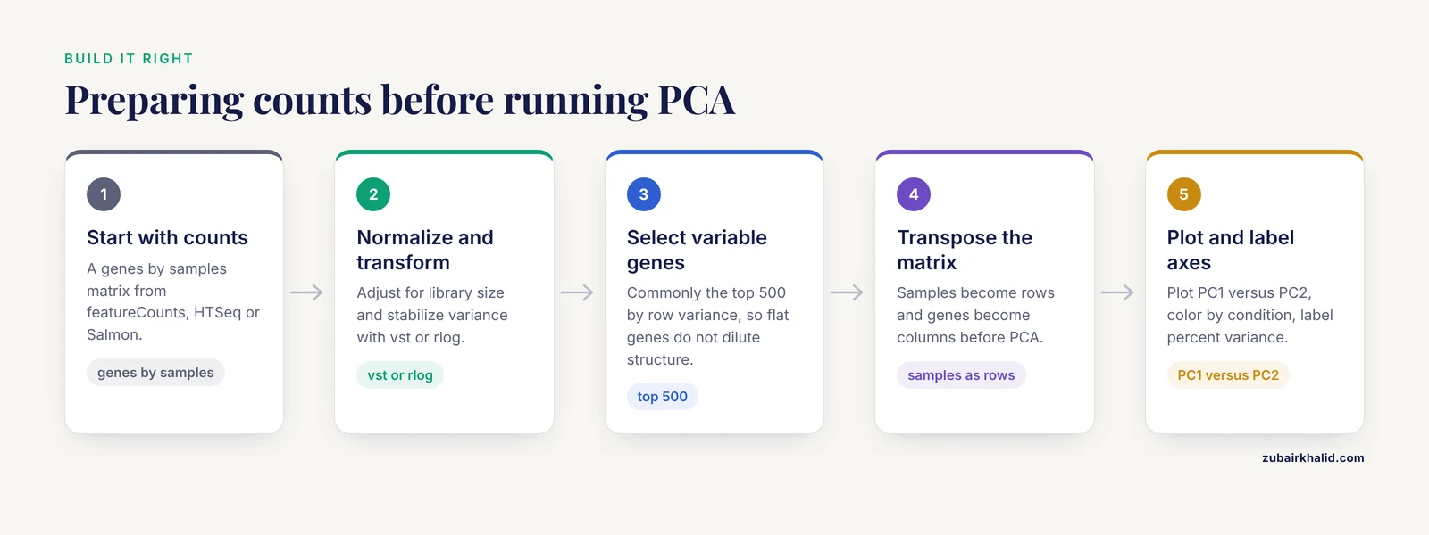
Principal component analysis is a dimensionality reduction technique. Given a matrix of samples by genes, it finds new axes (principal components) that capture the maximum variance in the data, in decreasing order. PC1 captures the largest source of variation, PC2 the second largest, and so on. When you plot PC1 on the x-axis and PC2 on the y-axis, each point is one sample, and samples with similar expression profiles land close together.
The standard workflow in RNA-seq looks like this:
- Start with a count matrix (genes by samples) from a tool such as featureCounts, HTSeq, or Salmon.
- Normalize for library size and, in the case of methods like DESeq2's variance-stabilizing transformation (vst) or the regularized log transformation (rlog), stabilize the variance across the count range.
- Optionally select the most variable genes, commonly the top 500 by row variance, so that thousands of flat, uninformative genes do not dilute the structure.
- Run PCA on the transposed matrix (samples as rows, genes as columns).
- Plot PC1 versus PC2, color points by your condition of interest, and label the axes with the percent of variance each component explains.
In DESeq2, this is a few lines:
library(DESeq2)
vsd <- vst(dds, blind = FALSE)
plotPCA(vsd, intgroup = c("condition", "batch"))
To see the percent variance and build the plot manually:
rv <- rowVars(assay(vsd))
select <- order(rv, decreasing = TRUE)[seq_len(500)]
pca <- prcomp(t(assay(vsd)[select, ]))
percentVar <- round(100 * pca$sdev^2 / sum(pca$sdev^2), 1)
Two properties of PCA follow directly from this construction and explain most of the confusion around interpretation:
- PCA is unsupervised. The algorithm never sees your group labels. It finds the biggest variance directions whatever they are. If the biggest variance direction is batch, sex, RNA integrity, or sequencing lane, that is what PC1 will show, and your condition may be pushed to PC3, PC4, or nowhere visible.
- PCA is dominated by the largest variance sources. A strong technical effect affecting 30 percent of the variance will compress a real biological effect affecting 5 percent of the variance into a small offset or into lower components. The plot shows variance, not statistical significance.
What "No Separation" Means in Practice
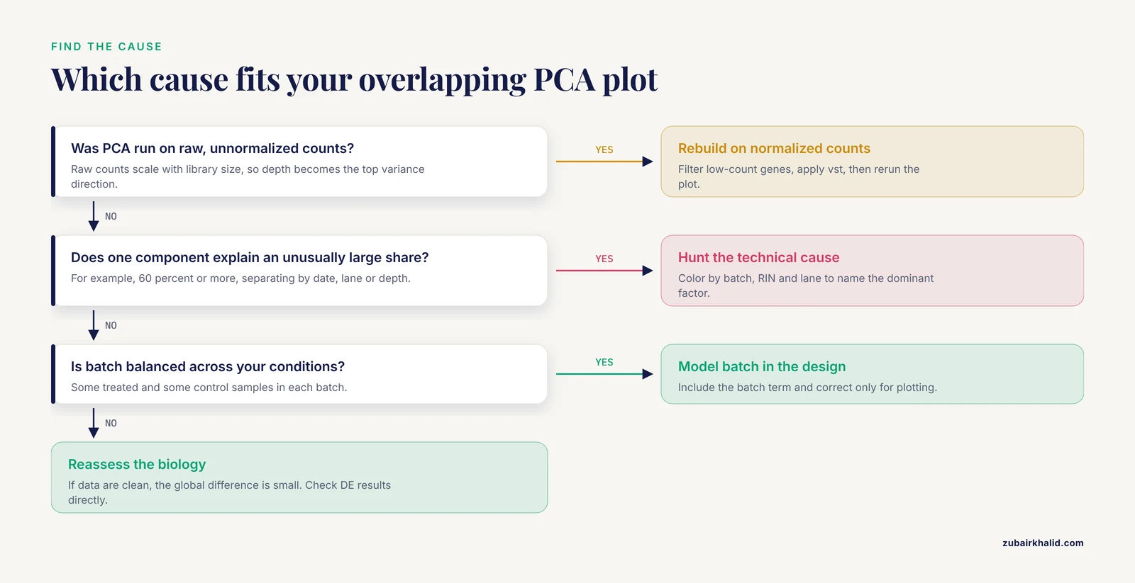
When a PCA plot shows no separation between groups, the points from both conditions overlap in the PC1 versus PC2 plane. There are five distinct situations that produce this picture, and they demand different responses.
1. The biological effect is small relative to other variation
This is the most common and most benign explanation. In a well-behaved dataset, the largest sources of variance are often individual-to-individual differences, batch, or cell-type composition, not the experimental condition. A treatment that changes 200 genes by 1.5-fold will produce a real but modest shift in expression space. If inter-individual noise or a batch effect explains 40 percent of the variance, that 1.5-fold shift may appear as a slight lean of one group toward the other, or as separation along PC3 or PC4 rather than PC1 or PC2.
The correct response is to look at more components. Plot PC3 versus PC4, or use a pairs plot of the first four to six components:
plotPCA(vsd, ntop = 500, pcX = 3, pcY = 4, intgroup = "condition")If the condition separates cleanly on PC3, the effect is real but smaller than the dominant noise sources. That is a normal finding in mammalian datasets with modest sample sizes.
2. There is genuinely no difference
Sometimes the biology is simply flat. A knockdown that failed, a drug that did not reach its target, a time point chosen before or after the response window, or a comparison between groups that truly do not differ will all produce overlapping PCA plots. In this case, the PCA result is honest and should be believed, especially if it is supported by other diagnostics: a sample-to-sample distance heatmap with no block structure, a volcano plot with no significant genes after correction, and no enrichment of your expected pathway.
3. A technical artifact dominates the data
If PC1 or PC2 explains an unusually large share of variance (for example, 60 percent or more) and the points separate by something other than your condition, such as sequencing date, library prep batch, flowcell lane, or read depth, then a technical factor is the dominant signal. When that factor is balanced across your conditions (some treated and some control samples in each batch), the condition effect can still be recovered statistically. When it is confounded with the condition (all controls in batch one, all treated in batch two), the batch effect and the condition effect are mathematically inseparable, and no amount of PCA or statistical modeling will fix the design. This is the single most serious interpretation of "no separation," because it can mean the experiment cannot answer the question it was built to answer.
4. The data were not prepared correctly for PCA
PCA on raw, unnormalized counts is a classic mistake. Raw counts scale with library size, so a sample sequenced at 20 million reads will look systematically different from one sequenced at 5 million reads, and that technical difference, not biology, becomes the top variance direction. Similarly, PCA on counts that include 15,000 low-count genes dominated by sampling noise will wash out real structure. The fix is to normalize, transform, and filter before running PCA, which is covered in the workflow section below.
5. The effect exists in genes that are not among the most variable
The default choice of the top 500 most variable genes is a convention, not a law. If your condition affects a small, coherent set of genes (for example, a transcription factor perturbation affecting a few dozen targets), those genes may not make the top 500 by variance, especially if the dataset has strong background variation. The separation then never appears on the plot even though differential expression testing will find it. Increasing ntop to 1,000 or 2,000, or running PCA on the genes that survive differential expression testing, can reveal structure that the default plot missed.
A Step-by-Step Troubleshooting Workflow
When a PCA plot shows no separation between groups, work through the following sequence. Each step is a concrete check with a concrete command, and each step either explains the overlap or moves you closer to the explanation.
Step 1: Confirm the plot was built correctly
Before interpreting anything, verify the input. The PCA should be run on normalized, variance-stabilized, filtered counts, not raw counts. In DESeq2:
dds <- DESeqDataSetFromMatrix(countData = cts, colData = coldata, design = ~ condition)
dds <- DESeq(dds)
keep <- rowSums(counts(dds) >= 10) >= 3   # keep genes with at least 10 counts in 3 samples
dds <- dds[keep, ]
vsd <- vst(dds, blind = FALSE)
plotPCA(vsd, intgroup = "condition")
The blind = FALSE argument matters when you have a design with a batch term, because it lets the transformation use the design. For a first look at the data before any modeling, blind = TRUE is the appropriate choice, because it does not let the expected condition effect influence the transformation. If you ran PCA on raw counts or on a matrix with thousands of near-zero genes, rebuild the plot first. A surprising number of "no separation" reports disappear at this step.
Step 2: Check library sizes and sequencing quality
Load the per-sample metrics from your alignment or quantification step into MultiQC and look at total reads, mapping rate, duplication rate, and gene body coverage. A sample with half the library size of the others, or a mapping rate 20 points below the rest, will distort the PCA. If one or two samples are technical outliers, they can pull the entire plot into a shape where the condition effect is invisible. Fix or flag those samples before drawing conclusions.
Step 3: Color the PCA by everything you know, not just the condition
Rebuild the plot with intgroup = c("condition", "batch"), then with intgroup = c("condition", "sex"), then with library preparation date, sequencing lane, RIN (RNA integrity number), or any other metadata you have. If the points separate by batch or by RIN rather than by condition, you have found the dominant variance source. If the points separate by nothing at all, the data may be genuinely homogeneous, which is good news for the model but means the condition effect is small.
Step 4: Look at a sample-to-sample distance heatmap
A heatmap of Euclidean distances between variance-stabilized samples, with hierarchical clustering, shows the same information as PCA in a different form:
sampleDists <- dist(t(assay(vsd)))
library(pheatmap)
pheatmap(sampleDists, clustering_distance_rows = sampleDists,
         clustering_distance_cols = sampleDists)
If the heatmap clusters samples by condition even though the PCA overlaps, trust the heatmap. If neither shows structure, the global expression profiles are similar across groups.
Step 5: Examine the lower principal components
Compute the percent variance for all components and plot PC1 through PC5 in pairs. A condition effect that explains 4 percent of the variance will not appear on a PC1 versus PC2 plot if batch explains 35 percent, but it will appear on PC3 or PC4. In DESeq2:
pcaData <- plotPCA(vsd, intgroup = "condition", returnData = TRUE)
percentVar <- round(100 * attr(pcaData, "percentVar"))
Then build the pairs plot manually from prcomp output. If the condition separates on PC3 with a clean margin, the effect is real and the analysis can proceed, with the caveat that the effect size is modest.
Step 6: Test whether the condition is associated with any component
A formal way to ask whether group labels correlate with PCA structure is a permutation test such as PERMANOVA (the adonis function in the R package vegan), applied to the sample distance matrix. This gives a p-value for the association between condition and overall expression variation, independent of which component carries it. If the test is significant but the PC1 versus PC2 plot overlaps, the effect is distributed across lower components, which confirms the interpretation from Step 5.
Step 7: Check for sample swaps and metadata errors
If one or two samples from one group sit inside the other group's cluster, suspect a sample swap or a mislabeled tube. Concrete checks include:
- Correlating each sample's expression of known marker genes with its recorded metadata (for example, sex markers such as XIST on the X chromosome, or tissue-specific markers).
- Comparing genotypes if the samples carry known variants.
- Checking whether the outlier samples share a batch, a lane, or a library prep date with the wrong group.
A single swapped sample can erase a visible separation. Correcting the metadata and rerunning the plot is often the entire fix.
Step 8: Address batch effects that are balanced across conditions
If batch is a real variance source but is balanced (each condition has samples in each batch), include the batch term in the design:
dds <- DESeqDataSetFromMatrix(cts, coldata, design = ~ batch + condition)The differential expression model will then control for batch even though the PCA plot still shows it. If you want to remove batch effects from visualization, DESeq2's removeBatchEffect (from the limma package) can be applied to the variance-stabilized matrix for plotting purposes only:
library(limma)
assay(vsd) <- removeBatchEffect(assay(vsd), vsd$batch)
plotPCA(vsd, intgroup = "condition")
Never use batch-corrected values for the differential expression test itself. Use the design matrix for testing and the corrected values for plotting.
Step 9: Recognize confounded designs
If all controls were processed in batch one and all treated samples in batch two, the design is confounded. The condition effect and the batch effect are perfectly correlated, and neither PCA, nor surrogate variable analysis, nor any statistical model can separate them. The honest options are to acknowledge the limitation, to treat the analysis as exploratory, or to repeat the experiment with a balanced design. Tools such as sva or RUVSeq can sometimes recover signal from partially confounded designs, but they cannot recover a fully confounded one.
Step 10: Reassess the biology
If the data are clean, normalized, filtered, and free of dominant artifacts, and the PCA still shows no separation, the remaining explanation is that the global expression difference between groups is small. At that point, look at the differential expression results directly. A dataset can have a handful of significant genes with modest fold changes and still show an overlapping PCA plot, because PCA reflects genome-wide variance while the test reflects per-gene signal. If the tests are also empty, the PCA was telling the truth: the groups do not differ detectably under these conditions, and the experiment should be redesigned (different time point, different dose, larger sample size, or a more sensitive comparison such as paired samples).
How This Compares to Other Diagnostic Plots
Analysts often confuse a PCA plot with the other standard RNA-seq diagnostics. The table below separates what each one shows and what "no separation" or "no signal" means in each.
| Plot or method | What it shows | What "no separation" means there | What it does NOT show |
|---|---|---|---|
| PCA plot (PC1 vs PC2) | The two largest variance directions in the data | The dominant variance sources are not aligned with your condition | Whether any individual genes are differentially expressed |
| MDS plot | Same information as PCA but using pairwise distances instead of eigen-decomposition | Same interpretation as PCA | Statistical significance |
| Sample distance heatmap | Pairwise similarity between all samples | Global expression profiles are similar across groups | Which genes drive the similarity |
| Volcano plot | Per-gene fold change versus per-gene significance | No genes pass the significance threshold | Whether the experiment was technically sound |
| Heatmap of top DE genes | Expression of the genes that passed testing | No genes passed testing, or the selected genes do not vary | Genome-wide structure |
| UMAP or t-SNE | Nonlinear embedding, often used in single-cell analysis | Local structure is absent, but distances are not quantitative | Reliable variance proportions |
The key distinction is between global and gene-level views. PCA asks whether the samples as a whole differ. A volcano plot asks whether any individual genes differ. These can disagree in both directions. A dataset can show clean PCA separation with no individually significant genes (many small coordinated shifts), or significant genes with no PCA separation (a few genes changing against a flat background). Neither plot alone is a verdict.
Common Mistakes and Limitations
The following mistakes account for most of the confusion around PCA plots with no separation. Each one is a concrete error with a concrete fix.
Running PCA on raw counts. Raw counts are proportional to library size. The top variance direction will reflect sequencing depth, not biology. Always normalize and transform first.
Interpreting an unsupervised plot as a hypothesis test. PCA produces no p-value. An overlapping plot does not prove the null hypothesis, and a separated plot does not prove the alternative. The statistical test for group differences is the differential expression model, not the PCA.
Coloring only by condition. If you color the points by condition and see nothing, you have not checked whether the data have structure. Color by batch, date, RIN, sex, and every other recorded variable. Structure that is invisible against one label may be obvious against another.
Ignoring the percent variance on the axes. A PC1 that explains 70 percent of the variance is telling you something different from a PC1 that explains 12 percent. Always read the axis labels. If PC1 explains a huge share and does not align with your condition, hunt for the technical cause.
Assuming the top 500 genes are the right gene set. The default is a convention. If a small set of genes carries the effect, it may not be in the top 500. Try larger ntop values, or run PCA on the genes that survive differential expression testing.
Deleting samples to force separation. Removing samples because they make the plot overlap is a form of p-hacking. Remove samples only for documented technical reasons, such as a failed library, a mapping rate far below the rest, or a confirmed sample swap.
Treating a confounded design as a statistical problem. If batch and condition are perfectly confounded, no analysis can separate them. This is a design limitation, not a bioinformatics troubleshooting problem, and it should be caught before sequencing, not after.
Expecting PCA to work the same in single-cell data. In single-cell RNA-seq, PCA is run on thousands of cells, often after feature selection and scaling, and the first 30 to 50 components are typically used for downstream clustering rather than the first two for plotting. The rules of interpretation differ enough that the two use cases should not be conflated.
Forgetting the individual-case caveat. Every dataset has its own design, its own metadata, and its own failure modes. The workflow above is a general diagnostic sequence, and unusual datasets deserve review by an experienced analyst before any conclusion is drawn.
Quick Review
- A PCA plot with no separation between groups means the top two variance directions do not align with your condition labels, not that the groups are identical.
- PCA is unsupervised. It never sees your group labels, so it shows the largest variance sources whatever they are.
- Always run PCA on normalized, variance-stabilized, filtered counts. Raw counts produce plots dominated by library size.
- Read the percent variance on the axes. A PC1 explaining most of the variance without aligning with your condition points to a technical artifact.
- Check lower components (PC3, PC4) and a sample distance heatmap before concluding there is no signal.
- A balanced batch effect can be modeled in the differential expression design. A confounded batch effect cannot be fixed after the fact.
- No separation on PCA is compatible with significant differential expression, and clean separation is compatible with no significant genes. The two views answer different questions.
Frequently Asked Questions
Does no separation in a PCA plot mean there are no differentially expressed genes?
No. PCA is unsupervised and reflects genome-wide variance, so a small set of differentially expressed genes can be invisible on the plot. Run the differential expression model and check the results directly. The PCA and the gene-level test answer different questions.
Should I run PCA on raw counts or normalized counts?
Normalized counts, always. Raw counts scale with library size, so sequencing depth becomes the dominant variance direction and the plot reflects technical artifacts rather than biology. Use a variance-stabilizing transformation such as DESeq2's vst, and filter out low-count genes before running PCA.
How many samples do I need for a PCA plot to be meaningful?
There is no fixed threshold, but with very few samples per group (two or three), PCA has little power to resolve a modest biological effect against individual noise. Larger sample sizes make the group structure easier to see and make the percent variance estimates more stable.
What should I do if PC1 separates by batch instead of my condition?
First confirm the batch is balanced across your conditions. If it is, include the batch term in the differential expression design and use batch-corrected values only for visualization. If the batch is confounded with the condition, the effects cannot be separated statistically, and the experiment needs to be repeated with a balanced design.
Is it an error if PC1 and PC2 together explain only 20 percent of the variance?
Not by itself. In noisy mammalian datasets, the first two components often explain a modest share of the variance, and that is normal. The concern arises only when a single component explains an unusually large share and does not align with your condition, which suggests a dominant technical artifact.
Can I use PCA on single-cell RNA-seq data the same way?
No. Single-cell PCA is typically run on thousands of cells after feature selection and scaling, and the first 30 to 50 components are used for clustering rather than the first two for a group comparison plot. The interpretation rules differ, and the two use cases should be treated separately.