How to Create a Parameterized R Markdown Report for RNA-Seq Analysis

By Dr. Zubair Khalid, DVM, MS, PhD · 2026-11-11

By the end of this guide you will be able to build a single parameterized R Markdown report that runs a complete differential expression workflow on any RNA-seq count matrix, then render a separate polished HTML or PDF report for each contrast, cutoff, or dataset you care about, all from one command. You will need R (4.2 or newer is a sensible baseline), the rmarkdown package, a TeX distribution if you want PDF output, and an RNA-seq count table with matching sample metadata. Everything else is installed from CRAN and Bioconductor, the open-source software repository for genomic analysis in R, using the commands shown below.

The core idea is simple. Instead of copying an analysis script five times and editing the comparison line in each copy, you write the analysis once and turn the variable parts, such as the count file path, the contrast, and the false discovery rate cutoff, into named parameters declared in the document header. Each rendered report records the exact values it ran with, which is precisely the kind of explicit methodological documentation that RNA-seq studies have historically lacked. A survey of RNA-seq methodology reporting found that papers routinely omit the pipeline details and reference choices needed to reproduce their results, and the authors argue for a standardized, explicit display of methodological information in every RNA-seq experiment [1]. A parameterized report is the most direct way to enforce that standard on your own work.

Why parameterize an RNA-seq report

Reproducibility in genomics is not an abstract virtue, it is an engineering constraint. The H3ABioNet consortium, which supports 27 research institutions across 17 African countries, built its variant calling, 16S, genotyping, and imputation workflows specifically because scalable, reproducible, portable, and easy-to-use analysis workflows are difficult to achieve with ad hoc scripts on heterogeneous computing environments [2]. The same lesson appears across bioinformatics. Longitudinal studies of workflow reuse note that small pipelines written as one-off scripts serve a single user well but do not scale into shareable, maintainable, reusable assets, which is why scientific workflow systems and literate programming tools exist in the first place [3].

A parameterized R Markdown file sits in the sweet spot between a bare script and a full workflow engine. R Markdown is a document format that interleaves narrative text with executable R code chunks, and knitr, the engine behind it, executes those chunks and weaves the results, tables, and figures into the final document. When you declare parameters in the YAML header, the small metadata block at the top of the file, every rendered output becomes a self-documenting record of one run. Reviewers, collaborators, and your future self can see which contrast produced which volcano plot.

Two failure modes push people toward this pattern. The first is workflow decay, the term one mass spectrometry group coined for analyses that become impossible to reproduce because they depend on a too-specific, undocumented computing platform [4]. The second is silent divergence, where five near-identical scripts drift apart as each gets edited for a different project. Surveys of RNA-seq reproducibility show that pipeline choices and parameterization introduce biases that biological replicates cannot absorb, so recording them is not optional bookkeeping, it is part of the result [1]. Modern protocol papers in genomics now bake harmonized parameterization and explicit reporting of intermediate outputs into their workflows as first-class design goals [5].

What you need installed

Work through this checklist before writing any code. All commands go into the R console.

R and RStudio. Install R from CRAN, then RStudio Desktop if you want the graphical Knit buttons. R works fine from the terminal alone, and on a cluster you will use the terminal.

rmarkdown and pandoc. RStudio bundles pandoc, the document converter that turns rendered Markdown into HTML, PDF, and Word. On a server or cluster without RStudio, install pandoc separately or let the rmarkdown package use its bundled copy.

install.packages("rmarkdown")

Bioconductor packages. Bioconductor is the standard repository for R genomics software, and a Bioconductor tutorial approach works for any of these installs. The BiocManager package handles installation.

if (!requireNamespace("BiocManager", quietly = TRUE)) {
    install.packages("BiocManager")
}
BiocManager::install(c(
    "DESeq2",
    "edgeR",
    "tximport",
    "EnhancedVolcano",
    "ComplexHeatmap"
))

DESeq2 performs differential expression testing on raw counts with a negative binomial model. edgeR is the other widely used count-based option, and published repositories of uniformly processed RNA-seq counts, such as Digital Expression Explorer 2 with more than 5.3 trillion assigned reads from 580,000 datasets, explicitly guarantee compatibility with both [6]. tximport imports transcript-level quantifications from tools like Salmon or kallisto and summarizes them to gene level. EnhancedVolcano draws volcano plots and ComplexHeatmap draws annotated heatmaps.

A test dataset. Any gene by sample count matrix in tab-separated format works. For a quick smoke test you can download gene-level counts for a public dataset from a repository such as DEE2, which serves counts programmatically through an R package, or use counts from your own featureCounts or Salmon run [6].

Input data layout. Two files:

• counts.tsv, genes as rows, samples as columns, gene identifiers in the first column.
• metadata.tsv, samples as rows, at least one column describing the condition you want to contrast.

Understanding the parameterized R Markdown format

A parameterized R Markdown document has three parts. The YAML header declares output format and parameters. Prose sections explain the analysis. Code chunks, fenced with triple backticks and marked {r}, do the work. The parameterized rmarkdown rna-seq format looks like this in miniature:

---
title: "[RNA-seq differential expression](/knowledge/bioinformatics/rna-seq-differential-expression-deseq2-edger) report"
output:
  html_document:
    toc: true
    toc_float: true
params:
  counts_file: "counts.tsv"
  metadata_file: "metadata.tsv"
  contrast_var: "condition"
  ref_group: "control"
  test_group: "treated"
  fdr_cutoff: 0.05
  lfc_cutoff: 1
  species: "human"
---

knitr::opts_chunk$set(echo = TRUE, warning = FALSE, message = FALSE)

Each entry under params becomes an R object named params inside the document, a list you access as params$counts_file, params$fdr_cutoff, and so on. When knitr renders the file, it injects the values you pass at render time, overriding the defaults shown in the header. The defaults are not decoration, they are the values used when someone clicks Knit without specifying anything, so choose them to match your most common case.

One chunk option matters enormously for parameterized reports. Setting params = "eval" in knitr::opts_chunk$set tells RStudio to substitute parameter values during interactive development rather than throwing errors because params does not exist yet. Add this to your setup chunk:

knitr::opts_chunk$set(echo = TRUE, warning = FALSE, message = FALSE)

Wait, that is the standard set. The parameter-aware version is:

knitr::opts_chunk$set(
    echo = TRUE,
    warning = FALSE,
    message = FALSE,
    params = "eval"
)

Hmm, one correction. The params = "eval" trick is a documented knitr feature, but the more robust habit is simply to reference params$... only inside chunks and to test interactively by sourcing a line that defines a local params list. Both approaches appear in real pipelines. Pick one and stay consistent.

Building the template, step by step

Create a file named rnaseq_report.Rmd. The following walkthrough builds it piece by piece.

Step 1. Write the YAML header with your parameters

This is the parameter block for a full differential expression report. Every parameter has a default so the file knits standalone.

---
title: "RNA-seq differential expression report"
subtitle: "A parameterized Bioconductor analysis"
author: "Computed automatically"
date: "`r Sys.Date()`"
output:
  html_document:
    toc: true
    toc_depth: 2
    number_sections: true
params:
  counts_file: "counts.tsv"
  metadata_file: "metadata.tsv"
  sample_col: "sample_id"
  contrast_var: "condition"
  ref_group: "control"
  test_group: "treated"
  covariates: NULL
  fdr_cutoff: 0.05
  lfc_cutoff: 1
  top_n: 25
  species: "human"
---

knitr::opts_chunk$set(echo = TRUE, warning = FALSE, message = FALSE)

A few of these deserve explanation. covariates holds optional batch variables such as batch or sex that enter the DESeq2 design formula. fdr_cutoff is the adjusted p-value threshold, conventionally 0.05, meaning you accept a 5 percent false discovery rate among the genes you call significant. lfc_cutoff is the minimum absolute log2 fold change you consider biologically interesting, and a value of 1 corresponds to a two-fold change.

Step 2. Record the run parameters in the output

The single most valuable chunk in the document prints the parameters back to the reader. This directly addresses the reproducibility gap documented for RNA-seq methodology reporting [1].

params_df <- data.frame(
    Parameter = names(params),
    Value = sapply(params, function(x) paste(deparse(x), collapse = " ")),
    row.names = NULL
)
knitr::kable(params_df, caption = "Parameters used for this run")

Rendered output looks like a two-column table listing counts_file with counts.tsv, fdr_cutoff with 0.05, and every other parameter beside its value.

Step 3. Load libraries and read the inputs

library(DESeq2)
library(EnhancedVolcano)
library(ComplexHeatmap)
library(circlize)

counts <- read.delim(params$counts_file, row.names = 1, check.names = FALSE)
meta   <- read.delim(params$metadata_file, stringsAsFactors = FALSE)

Make sure the count columns and metadata rows line up in the same order. Do not rely on file order, enforce it.

rownames(meta) <- meta[[params$sample_col]]
stopifnot(setequal(colnames(counts), rownames(meta)))
meta <- meta[colnames(counts), , drop = FALSE]

The stopifnot() line is your cheapest quality control checkpoint. If sample names mismatch, the report fails immediately with a clear cause rather than producing a subtly wrong result downstream. Structured checkpoints like this one, placed between every major stage, are a hallmark of well-designed reproducible pipelines in current genomics protocols [5].

Step 4. Build the design formula from parameters

if (is.null(params$covariates)) {
    design_formula <- as.formula(paste("~", params$contrast_var))
} else {
    design_formula <- as.formula(
        paste("~", paste(c(params$covariates, params$contrast_var),
                         collapse = " + "))
    )
}
design_formula

For the defaults this evaluates to ~ condition. With covariates: ["batch", "sex"] it becomes ~ batch + sex + condition, which adjusts the test for those sources of variation.

Step 5. Run DESeq2

meta[[params$contrast_var]] <- factor(
    meta[[params$contrast_var]],
    levels = c(params$ref_group, params$test_group)
)
dds <- DESeqDataSetFromMatrix(
    countData = round(as.matrix(counts)),
    colData   = meta,
    design    = design_formula
)
dds <- dds[rowSums(counts(dds)) >= 10, ]
dds <- DESeq(dds)
res <- results(dds, contrast = c(params$contrast_var,
                                 params$test_group,
                                 params$ref_group))
res_df <- as.data.frame(res)
res_df$gene <- rownames(res_df)

Two details carry the parameterization. Setting factor levels with the reference group first fixes which direction log2 fold changes point, positive means up in test_group relative to ref_group. The contrast = argument to results() names the groups explicitly so the report is unambiguous months later. The prefiltering step, keeping genes with at least 10 total reads, is standard practice to reduce the multiple-testing burden on genes with too little information to test.

Step 6. Summarize and visualize

sig <- subset(res_df, padj < params$fdr_cutoff &
              abs(log2FoldChange) > params$lfc_cutoff)
up   <- subset(sig, log2FoldChange > 0)
down <- subset(sig, log2FoldChange < 0)
knitr::kable(
    data.frame(
        Comparison = paste(params$test_group, "vs", params$ref_group),
        FDR_cutoff = params$fdr_cutoff,
        LFC_cutoff = params$lfc_cutoff,
        Upregulated = nrow(up),
        Downregulated = nrow(down)
    ),
    caption = "Differential expression summary"
)

EnhancedVolcano(
    res_df,
    x = "log2FoldChange",
    y = "padj",
    lab = res_df$gene,
    pCutoff = params$fdr_cutoff,
    FCcutoff = params$lfc_cutoff,
    title = paste(params$test_group, "vs", params$ref_group),
    subtitle = NULL
)

top_genes <- head(
    res_df[order(res_df$padj), "gene"],
    params$top_n
)
mat <- log2(counts(dds, normalized = TRUE)[top_genes, ] + 1)
Heatmap(
    mat,
    name = "log2 norm counts",
    col = colorRamp2(c(0, max(mat)), c("white", "firebrick")),
    column_title = paste("Top", params$top_n, "genes by adjusted p-value")
)

Notice how top_n flows straight from the header into the heatmap. Change one parameter, render again, and the figure updates without you touching a line of analysis code.

Step 7. Write out a results table

out_name <- paste0(
    "DE_results_", params$test_group, "_vs_", params$ref_group, ".tsv"
)
write.table(res_df, out_name, sep = "\t", quote = FALSE, row.names = FALSE)

The filename embeds the contrast, so rendering several reports never overwrites a previous result. This habit of naming intermediate outputs by their parameters is one of the explicit reporting practices that recent genomics protocols highlight as central to transparency [5].

Rendering the report

The basic render call

From the R console, in the directory containing the file:

rmarkdown::render(
    "rnaseq_report.Rmd",
    params = list(
        counts_file   = "counts.tsv",
        metadata_file = "metadata.tsv",
        contrast_var  = "condition",
        ref_group     = "control",
        test_group    = "treated",
        fdr_cutoff    = 0.05,
        lfc_cutoff    = 1
    ),
    output_file = "report_treated_vs_control.html"
)

Expected console output:

processing file: rnaseq_report.Rmd
  |..............                                          |  25%
  ordinary text without R code

  |............................                            |  50%
label: setup (with options)
list of 2
  $ include: logi FALSE
  $ params : chr "eval"

output file: report_treated_vs_control.html

RStudio also offers a graphical path. Click the Knit dropdown next to the Knit button and choose Knit with Parameters, or press Ctrl+Shift+K on Windows and Linux, Cmd+Shift+K on macOS. A dialog opens with one field per parameter, prefilled with the defaults. This is the fastest way to explore, while the programmatic render() call is what you script.

Rendering one report per contrast

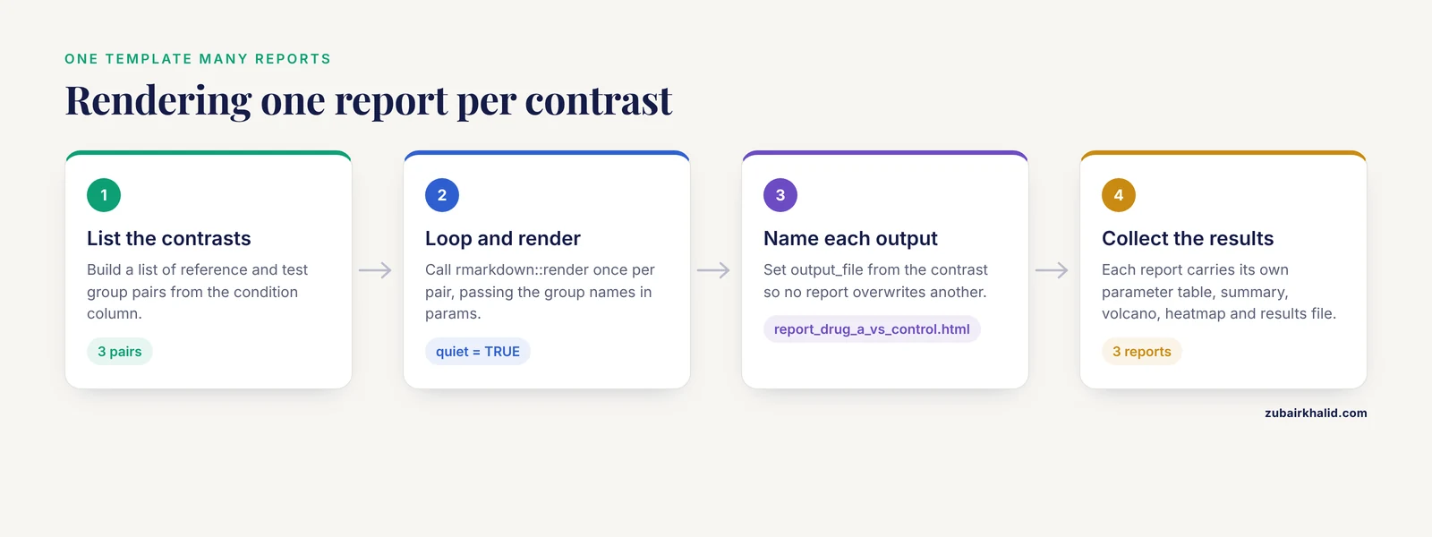
The payoff of the parameterized rmarkdown rna-seq template arrives when you loop it. Suppose your metadata has a condition column with three levels, control, drug_a, and drug_b.

contrasts <- list(
    c("control", "drug_a"),
    c("control", "drug_b"),
    c("drug_a",  "drug_b")
)

for (ct in contrasts) {
    rmarkdown::render(
        "rnaseq_report.Rmd",
        params = list(
            counts_file   = "counts.tsv",
            metadata_file = "metadata.tsv",
            contrast_var  = "condition",
            ref_group     = ct[2],
            test_group    = ct[1],
            fdr_cutoff    = 0.05,
            lfc_cutoff    = 1
        ),
        output_file = paste0("report_", ct[1], "_vs_", ct[2], ".html"),
        quiet = TRUE
    )
}

Three self-contained reports, each with its own parameter table, summary, volcano plot, heatmap, and results file, generated without a single copy-pasted script. For longer job lists, read the contrast combinations from a spreadsheet and pass each row in, or use purrr::pwalk() to drive render() over a data frame of parameter sets. When the number of reports grows large, the same loop runs on a high-performance computing cluster as an array job, which is exactly the scaling boundary where workflow researchers note that hand-run R scripts stop being enough and structured pipelines take over [3].

Rendering to PDF or Word

Change the output format by passing output_format to render(). PDF output requires a LaTeX installation, typically TinyTeX, which you can install with tinytex::install_tinytex().

rmarkdown::render(
    "rnaseq_report.Rmd",
    output_format = "pdf_document",
    params = list(counts_file = "counts.tsv",
                  metadata_file = "metadata.tsv",
                  contrast_var = "condition",
                  ref_group = "control",
                  test_group = "treated"),
    output_file = "report_treated_vs_control.pdf"
)

Extracting the bare R code

When a collaborator wants the script without the prose, knitr::purl() extracts every code chunk into an R file:

knitr::purl("rnaseq_report.Rmd", "rnaseq_analysis.R", documentation = 0)

Parameter reference table

The parameters in this template, their types, purposes, and example values:

Common errors and their fixes

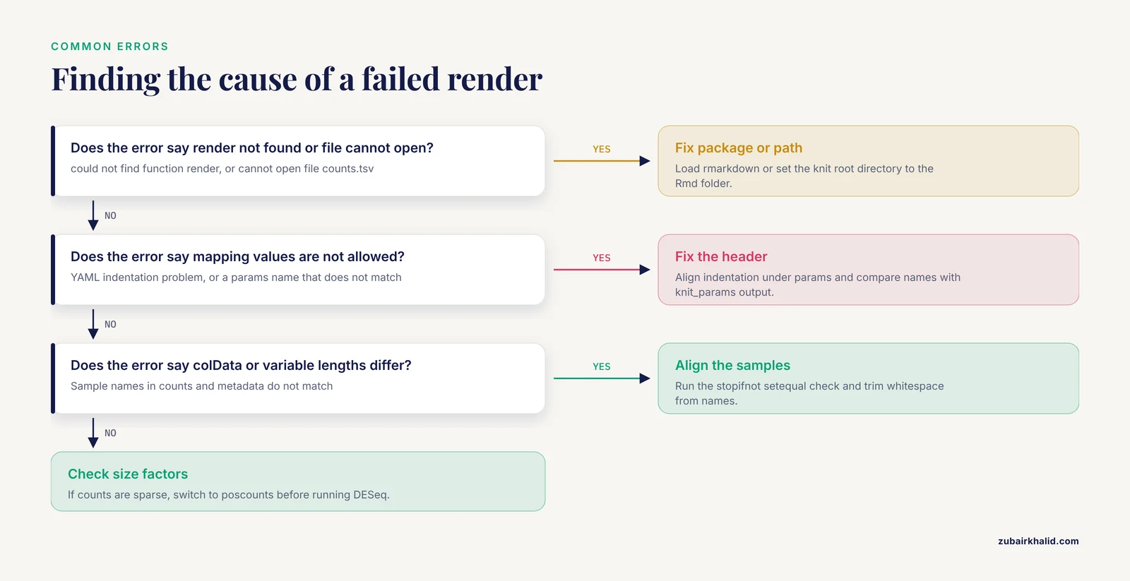
These are the failures you will actually hit, with the exact messages and what to do.

Error: could not find function "render". You called render() without loading the package. Run library(rmarkdown) or use the fully qualified rmarkdown::render() as shown above.

Error in yaml::yaml.load(..., error.label = ...): mapping values are not allowed here. Your YAML header has an indentation problem. YAML is whitespace sensitive, so each params entry must sit at the same indent level under params: with a single space after each colon. Convert a numeric-looking string by quoting it, because sample_id: 001 becomes the number 1 while sample_id: "001" stays a string.

Error in read.delim(...): cannot open file 'counts.tsv'. The path is relative to the directory where rendering starts, not where the Rmd file lives. Two fixes. Either setwd() to the project directory before rendering, or, better, add this chunk so knitr treats the Rmd file's folder as the working directory:

knitr::opts_knit$set(root.dir = normalizePath("../"))

Error in estimateSizeFactorsForMatrix(counts(object), ...) : every gene contains at least one zero, cannot compute log geometric means. DESeq2's default size factor estimation needs genes with nonzero counts across all samples, which fails on very sparse single-cell-like matrices. Switch to dds <- estimateSizeFactors(dds, type = "poscounts") before running DESeq(), or prefilter more aggressively.

Error in DESeqDataSetFromMatrix(...) : some columns in colData are not in countData or variable lengths differ. Sample names in metadata and count columns do not match. The stopifnot(setequal(...)) alignment chunk from Step 3 catches this before it happens. Check for hidden whitespace with colnames(counts) printed alongside rownames(meta), and clean names with trimws() if needed.

all genes have equal values from DESeq2. Your count matrix is degenerate, often caused by reading a file where genes are columns and samples are rows. Transpose it or fix the import so genes are rows.

Error: pandoc version 1.12.3 or higher is required and was not found. The machine has no usable pandoc. Install it with install.packages("rmarkdown") on desktop systems, which fetches a bundled copy, or install pandoc through your system package manager on Linux servers.

object 'params' not found while testing chunks interactively. The params object only exists during knit. For interactive development, define a local list in a chunk you later delete or guard with if (knitr::is_interactive()), for example params <- list(counts_file = "counts.tsv", fdr_cutoff = 0.05).

Warning: The 'params' argument does not match any declared parameter. You passed a name in the params list that does not appear in the YAML header, usually a typo like counts_file versus count_file. Compare against knitr::knit_params("rnaseq_report.Rmd"), which prints every declared parameter and its default.

Verifying the report is correct

Check four things after every render. First, open the HTML and confirm the parameter table at the top matches the run you intended, because a report rendered with the wrong contrast is worse than no report. Second, confirm the sample counts line up, with the number of count columns equal to the number of metadata rows and both matching your design. Third, look at the size factor spread and a principal component plot before trusting fold changes. A PCA colored by your contrast variable tells you whether the biology dominates or a batch effect does. Fourth, spot-check one gene by hand, comparing its normalized counts across groups with the reported log2 fold change. A two-fold upregulation means the treated group's normalized mean counts are roughly twice the control group's, which you can verify with:

round(
    tapply(counts(dds, normalized = TRUE)["GENE_OF_INTEREST", ],
           meta[[params$contrast_var]], mean),
    1
)

Also verify that the exported results file opens cleanly and that its row count equals the number of genes tested, which is printed in the DESeq2 output as the number of rows remaining after prefiltering.

Scaling up and integrating with workflows

A parameterized report is a component, not a ceiling. Three directions extend it naturally.

Wrap it in a workflow engine. When a pipeline must run on clusters, handle large data volumes, and be reused across projects, the consensus in the workflow engineering literature is that plain R scripts and notebooks stop being sufficient and scientific workflow systems earn their keep [3]. A parameterized Rmd renders cleanly from a Snakemake or Nextflow rule, with the workflow passing file paths and contrasts as parameters. The tcga-data-nf project shows the pattern at scale, using a Nextflow workflow to download, preprocess, and analyze RNA-seq and methylation data from thousands of TCGA samples with a single command, backed by an R companion package for data management [7]. Your Rmd plays the role their R package plays, the analyzed step inside a larger reproducible shell.

Version and share it. Put the template under version control with the parameters documented in the README. The GCAC project demonstrates the same composition from the other direction, an R-based analysis pipeline wrapped in Galaxy so that researchers get literate, reproducible outputs through a web interface [8]. Publishing your template with a working example dataset turns it from personal convenience into a reusable contribution.

Prefer preprocessed counts where appropriate. Not every project needs raw fastq processing inside the report. Repositories of uniformly processed gene-level counts, such as DEE2, let a parameterized report start directly from a counts matrix while keeping consistency across experiments, and their data are designed for exactly the edgeR and DESeq2 style analyses shown here [6]. This keeps the report fast and focused on the statistical question.

Common Mistakes and Limitations

• Hardcoding values inside chunks while also declaring them as parameters. If a chunk contains res <- results(dds, contrast = c("condition", "treated", "control")) while the header declares contrast_var, rendering with different parameters silently ignores them. Every analysis decision that varies between runs must read from params$.
• Forgetting that the Knit button uses defaults, not your last render call. RStudio's plain Knit runs with header defaults. Use Knit with Parameters for interactive variation and rmarkdown::render() for scripted runs.
• Treating fold change direction as interchangeable. Sign depends entirely on factor level order. Always set the reference group explicitly and print the comparison direction in the report, as the template does in the summary table.
• Ignoring batch structure. A parameterized report makes it easy to render twenty contrasts quickly, and it makes it just as easy to render twenty wrong ones if a batch effect confounds the design. Inspect the PCA and include relevant covariates in covariates.
• Overfitting the template to one dataset. A template full of dataset-specific assumptions, such as hardcoded gene filters or species-specific annotation, defeats the purpose. Keep dataset-specific decisions in parameters or in a separate preprocessing script.
• Expecting the report to substitute for raw data provenance. A parameterized document records the statistical analysis, not the upstream sequencing, alignment, and quantification choices. Because RNA-seq methodology reporting has been shown to limit reproducibility when pipeline details go unspecified, document the upstream pipeline separately, including tool versions and reference genome [1].
• Long render times on every knit. If the DESeq2 fit takes an hour, cache expensive chunks with cache = TRUE and parameterize the cache path by contrast so runs do not collide.
• Finally, any biological conclusion from a differential expression analysis, particularly for clinical or animal-work decisions, needs review by a qualified investigator with domain knowledge of the study system, and no automated report replaces that judgment.

Frequently Asked Questions

Can I use the Knit button with parameters?

Yes, use the Knit dropdown and choose Knit with Parameters, or press Ctrl+Shift+K. A dialog appears listing every parameter from the YAML header with its default value filled in.

How do I render the same report for many contrasts at once?

Loop over a list of contrasts and call rmarkdown::render() once per combination, passing a distinct output_file name for each so results do not overwrite. The loop example in the rendering section produces three reports in one run.

Do I need R Markdown or should I use Quarto?

Both work for this pattern. Quarto, the newer publishing system from the same team, supports parameters with nearly identical syntax, and rmarkdown remains fully supported. If your team already has R Markdown infrastructure, stay with it, since a working parameterized rmarkdown rna-seq template is worth more than a format migration.

Where should the counts matrix come from?

From featureCounts, Salmon plus tximport, or a public repository of precomputed counts. DEE2 provides uniformly processed gene-level counts for hundreds of thousands of public datasets and is designed to feed straight into DESeq2 or edgeR [6].

How do I hide the R code from collaborators who only want results?

Set echo = FALSE in the chunk options, or use knitr::opts_chunk$set(echo = FALSE) globally in the setup chunk. Keep a second parameterized version with code visible for your own records.

Can I run parameterized reports on a compute cluster?

Yes. R and pandoc install fine on headless Linux systems, and rmarkdown::render() needs no GUI. Array jobs can call render with different parameter sets in parallel, one per contrast, which is how R-based report steps embed inside larger cluster workflows [3].

Why do my parameter values revert to defaults?

The Knit button and any render() call without a params argument use the YAML defaults. If you passed params but see defaults, check that the parameter names in the list exactly match the header, and confirm you are passing a list, not named arguments.

How do I share the finished report?

The rendered HTML file is self-contained, so email it, drop it in a shared drive, or post it with your repository. Including the parameter table in the report is what makes it interpretable to someone who did not run it, and for published work this explicit statement of methods and parameters is exactly the reporting standard the RNA-seq reproducibility literature calls for [1].

`

Sources

1. Current RNA-seq methodology reporting limits reproducibility
2. Developing reproducible bioinformatics analysis workflows for heterogeneous computing environments to support African genomics.
3. Developing and reusing bioinformatics data analysis pipelines using scientific workflow systems.
4. An evolving computational platform for biological mass spectrometry: workflows, statistics and data mining with MASSyPup64.
5. A Guide to Enzymatic Targeted Methylation Sequencing Bioinformatics Workflow: Best Practices.
6. Digital expression explorer 2: a repository of uniformly processed RNA sequencing data.
7. Reproducible processing of TCGA regulatory networks.
8. GCAC: galaxy workflow system for predictive model building for virtual screening.