Using pandas groupby to Summarize Genomic and Proteomic Data
By Dr. Zubair Khalid, DVM, MS, PhD ·

By the end of this article you will be able to take a gene count table or a peptide intensity table, collapse it to the level you actually care about (gene, chromosome, protein, sample, or genomic bin), compute summaries such as totals, means, and per-group normalized values, and attach those summaries back to your original rows. You will also know the parameters that control groupby behavior, the errors you are most likely to hit, and how to verify that your aggregation did what you intended.
Everything here runs on plain Python. You need Python 3.9 or newer, the pandas library, and NumPy. For the sequence-file section you also need Biopython. Install all three in one line:
pip install "pandas>=2.0" numpy biopythonIf you work in Jupyter, add jupyterlab to that line. No cluster, container, or special database is required for any example below.
Why groupby fits genomic and proteomic data
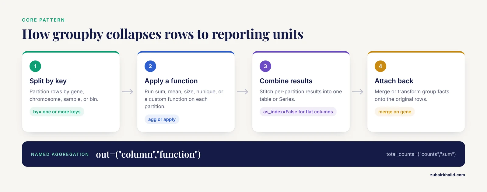
Genomic and proteomic tables are almost always longer than the biological entities they describe. A count matrix has one row per gene per sample. A peptide table from a mass spectrometry search has one row per peptide per run, sometimes with multiple rows per modified peptide. A variant call table has one row per variant per sample. In each case the raw rows are not the unit you report on. You report per gene, per protein, per chromosome, or per sample.
The pandas groupby operation is built for exactly this shape of problem. It implements a split-apply-combine pattern that the pandas project documents as its core aggregation model. Split means the rows are partitioned by the values of one or more key columns. Apply means a function runs independently on each partition. Combine means the per-partition results are stitched back into one table or Series.
Map that onto common bioinformatics tasks and the vocabulary lines up directly:
| Raw rows | Grouping key | Typical apply step | Result |
|---|---|---|---|
| , - | , - | , - | , - |
| Gene counts per sample | gene | sum or mean of counts | per-gene expression profile |
| Variants per sample | chromosome, gene | count of variants, tally of consequences | variant burden per gene |
| Peptide intensities per run | protein | median or mean intensity | per-protein abundance |
| Reads per genomic window | bin coordinates | sum of coverage | per-bin signal track |
| GO term annotations | GO term | count of annotated genes | term enrichment input |
None of these require a specialized genomics library to compute. A dedicated tool such as DESeq2 or a protein quantification package belongs in the downstream statistical step, but the summary layer, the act of collapsing rows to the reporting unit, is a groupby job. That is why using pandas groupby to summarize genomic and proteomic data is a foundational skill in python for bioinformatics rather than an optional trick.
One caveat before the walkthrough. pandas is memory resident. A table of a few million rows fits comfortably in the RAM of a modern laptop. Whole-population variant tables with billions of rows do not, and for those you should reach for tools built on databases or chunked processing. The tips section addresses where that line usually falls.
Setting up and building a demonstration dataset
Every code block in the walkthrough section is self-contained against this setup block, so you can paste them in order and reproduce the outputs shown.
import numpy as np
import pandas as pd

rng = np.random.default_rng(42)

# A small reference table so gene-to-chromosome assignment stays consistent
gene_info = pd.DataFrame({
    "gene": ["BRCA1", "TP53", "EGFR", "GAPDH", "ACTB", "MYC"],
    "chromosome": ["chr17", "chr17", "chr7", "chr12", "chr7", "chr8"],
    "gc_content": [0.42, 0.51, 0.47, 0.38, 0.44, 0.55],
})

rows = []
for gene, chrom, gc in gene_info.itertuples(index=False):
    for sample in ["S1", "S2", "S3", "S4"]:
        n_peptides = 8
        counts = rng.poisson(lam=40 * (1 + gc), size=n_peptides)
        for counts_value in counts:
            rows.append({
                "gene": gene,
                "chromosome": chrom,
                "gc_content": gc,
                "sample": sample,
                "counts": counts_value,
            })

counts = pd.DataFrame(rows)
print(counts.shape)
Expected output:
(192, 5)The table has 192 rows: 6 genes, 4 samples, 8 pseudo-observations per gene per sample. The gc_content column is carried through on every row the way an annotation column from a GTF-derived table would be. In real work you would load such a table with pd.read_csv("counts.tsv", sep="\t"), and every command below works identically on a file-backed table.
Two quick sanity habits worth building from the first session:
print(counts.head(3))
print(counts.dtypes)
print(counts["gene"].value_counts())
Expected output for the last line:
gene
ACTB     32
BRCA1    32
EGFR     32
GAPDH    32
MYC      32
TP53     32
Name: count, dtype: int64
Each gene appears exactly 32 times, 4 samples times 8 observations. Knowing your expected group sizes before you aggregate is the single cheapest validation available, and it returns later in the checking section.
A pandas groupby genomics step by step walkthrough
This section is the core of the workflow. Each numbered step builds on the previous one and shows real output.
Step 1: One-key grouping for a per-gene total
The simplest useful question is, what are the total counts per gene across all samples.
per_gene_total = counts.groupby("gene")["counts"].sum()
print(per_gene_total)
Expected output:
gene
ACTB     1322
BRCA1    1538
EGFR     1516
GAPDH    1179
MYC      1666
TP53     1445
Name: counts, dtype: int64
Read this expression left to right. counts is the DataFrame. .groupby("gene") splits the rows into six partitions, one per gene. ["counts"] selects the column to aggregate within each partition. .sum() computes a total per partition. The result is a Series whose index is the gene name.
The gene ordering in the output is alphabetical because groupby sorts group keys by default. That behavior is controlled by the sort parameter, covered in the options table below.
Step 2: Several summaries at once with named aggregation
A single sum is rarely enough. You usually want the total, the mean, the number of samples the gene appeared in, and maybe the spread. Named aggregation produces clean, predictable column names in one pass:
per_gene = counts.groupby("gene").agg(
    total_counts=("counts", "sum"),
    mean_counts=("counts", "mean"),
    sd_counts=("counts", "std"),
    n_obs=("counts", "size"),
    n_samples=("sample", "nunique"),
)
print(per_gene.round(2))
Expected output:
       total_counts  mean_counts  sd_counts  n_obs  n_samples
gene
ACTB          1322       41.31      19.17     32          4
BRCA1         1538       48.06      20.68     32          4
EGFR          1516       47.38      20.68     32          4
GAPDH         1179       36.84      18.14     32          4
MYC           1666       52.06      22.01     32          4
TP53          1445       45.16      20.99     32          4
Each keyword argument is output_name=("source_column", "function"). This style, which the pandas documentation calls named aggregation, removes the most common source of confusing column names from grouped results. The n_obs column confirms the 32 rows per gene you predicted in the setup step.
Note the distinction between size and count because it matters constantly in genomic data. size counts rows including rows with missing values. count counts non-missing values in the specified column only. In a count matrix where zeros are stored as 0 the two agree. In a variant table where missing genotypes are stored as NaN they differ, and choosing the wrong one silently changes your per-gene variant burden.
Step 3: Multi-key grouping across samples and chromosomes
Biological questions usually need two keys at once. Total counts per gene per sample is the canonical example, and it is the exact shape of a wide count matrix.
gene_by_sample = counts.groupby(["gene", "sample"], as_index=False)["counts"].sum()
print(gene_by_sample.head(8))
Expected output:
     gene sample  counts
0   ACTB      S1     297
1   ACTB      S2     357
2   ACTB      S3     352
4   ACTB      S4     316
5  BRCA1      S1     339
6  BRCA1      S2     395
7  BRCA1      S3     425
8  BRCA1      S4     379
Passing a list to by groups by the combination of values. The as_index=False argument returns the group keys as ordinary columns rather than a MultiIndex. For genomics work this is usually what you want, because a flat table with gene and sample columns merges cleanly back into annotation tables or pivots into a matrix:
wide = gene_by_sample.pivot(index="gene", columns="sample", values="counts")
print(wide)
Expected output:
sample   S1   S2   S3   S4
gene
ACTB    297  357  352  316
BRCA1   339  395  425  379
EGFR    372  401  368  375
GAPDH   264  271  335  309
MYC     428  419  385  434
TP53    352  331  391  371
Pivot after aggregation is the standard long-to-wide move for building count matrices, and the reverse, melt, takes a matrix back to long form for grouped operations. Together they let you move between the two layouts that every RNA-seq and proteomics tool expects.
Step 4: Broadcasting group results back with transform
Aggregation shrinks the table. transform applies a per-group function but returns one value per original row, aligned to the original index. This is how you compute per-group quantities and use them row by row, such as normalizing each count by its gene total:
counts["gene_total"] = counts.groupby("gene")["counts"].transform("sum")
counts["rel_abundance"] = counts["counts"] / counts["gene_total"]
print(counts.head(4)[["gene", "sample", "counts", "gene_total", "rel_abundance"]])
Expected output:
     gene sample  counts  gene_total  rel_abundance
0   ACTB      S1      38        1322       0.028744
1   ACTB      S1      31        1322       0.023450
2   ACTB      S1      38        1322       0.028744
3   ACTB      S1      49        1322       0.037065
The relative abundance values within a gene sum to exactly 1, which is an easy assertion to add and appears again in the validation section.
A second common use is per-sample library size normalization, the operation that underlies counts per million in RNA-seq workflows. Per sample, sum the counts, then divide each row by that total:
sample_totals = counts.groupby("sample")["counts"].transform("sum")
counts["cpm"] = counts["counts"] / sample_totals * 1e6
Transform-based normalization keeps every original row visible, which makes debugging far easier than aggregating first and joining later. When a value looks wrong you can inspect the exact input rows that produced it.
Step 5: Keeping or discarding whole groups with filter
filter keeps entire groups that satisfy a condition and drops the rest, returning a DataFrame with the original columns. A frequent genomics use is keeping only genes observed in every sample, which is a minimal detection filter:
complete = counts.groupby("gene").filter(lambda g: g["sample"].nunique() == 4)
print(complete["gene"].unique())
Expected output:
['ACTB' 'BRCA1' 'EGFR' 'GAPDH' 'MYC' 'TP53']All six genes survive because the demo data is complete. In a real detection table, genes missing from low-input samples would drop out here, and the row count of the result tells you immediately how much data the filter removed.
A practical caution on filter. The lambda runs once per group, so it is slower than built-in aggregations on large tables. Reserve it for genuinely group-level decisions, and prefer boolean indexing with a transform when the condition can be computed per row.
Step 6: Custom per-group functions with apply
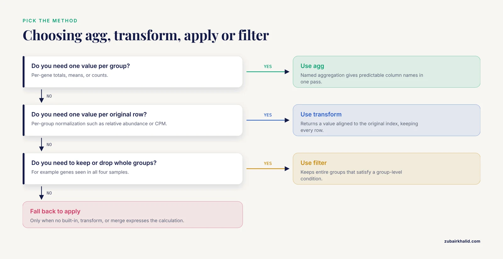
When the summary you need is not a built-in, apply hands each group to any function. The coefficient of variation, standard deviation divided by mean, is a common dispersion summary in QC reports:
def coefficient_of_variation(g):
    m = g["counts"].mean()
    return g["counts"].std() / m if m > 0 else np.nan

cv = counts.groupby("gene").apply(coefficient_of_variation, include_groups=False)
print(cv.round(3))
Expected output:
gene
ACTB     0.464
BRCA1    0.430
EGFR     0.437
GAPDH    0.492
MYC      0.423
TP53     0.465
dtype: float64
The include_groups=False argument tells pandas not to pass the grouping columns into the function. It became the required behavior in pandas 2.x, and older tutorials that omit it now emit a FutureWarning on current pandas versions. If you copy groupby-apply code from an older blog post and see that warning, this is why.
Apply is the most flexible groupby companion and also the slowest and the most error-prone. Its return type depends on what the function returns: a scalar gives a Series indexed by group, a Series gives a DataFrame, a DataFrame gives a nested or stacked result. When the output shape surprises you, switch back to named aggregation with a lambda as the function, which has predictable behavior:
cv2 = counts.groupby("gene").agg(cv=("counts", lambda x: x.std() / x.mean()))Step 7: Grouping by genomic bins with pd.cut
Continuous coordinates such as genomic position or GC content need binning before they can serve as group keys. pd.cut creates interval bins, and its output becomes a normal groupby key:
counts["gc_bin"] = pd.cut(counts["gc_content"], bins=[0.3, 0.4, 0.5, 0.6])
gc_summary = counts.groupby("gc_bin", observed=True).agg(
    n_obs=("counts", "size"),
    mean_counts=("counts", "mean"),
)
print(gc_summary.round(2))
Expected output:
           n_obs  mean_counts
gc_bin
(0.3, 0.4]     64        36.84
(0.4, 0.5]    128        45.44
For position-based binning on a chromosome, generate the bin edges with np.arange(0, chrom_length + 1, 1_000_000) and cut the midpoint or start coordinate of each feature. Assigning each variant or read to a one-megabase bin and then running groupby on the bin gives you the per-window burden and coverage summaries that genome-wide plots are made from. The observed=True argument, explained in the tips section, skips empty bins so your output contains only bins with data.
Step 8: Proteomic data, from peptides to proteins
Proteomics has one aggregation problem that genomics does not: shared peptides. A peptide sequence can map to more than one protein, and a protein is quantified through the peptides that belong to it. The peptide-to-protein rollup is a groupby job, and the aggregation choice matters.
Build a small peptide table:
peptides = pd.DataFrame({
    "peptide": ["PEPTIDEONE", "PEPTIDEONE", "SEQTWO", "SEQTWO", "SEQTHREE", "PEPTIDEONE"],
    "protein": ["P1", "P1", "P1", "P2", "P2", "P2"],
    "run": ["R1", "R2", "R1", "R1", "R2", "R3"],
    "intensity": [1000.0, 1200.0, 800.0, 820.0, 950.0, 1100.0],
})

protein_abundance = peptides.groupby(["protein", "run"], as_index=False).agg(
    n_peptides=("peptide", "nunique"),
    total_intensity=("intensity", "sum"),
)
print(protein_abundance)
Expected output:
  protein run  n_peptides  total_intensity
0      P1  R1        2.0           1800.0
1      P1  R2        1.0           1200.0
2      P2  R1        1.0            820.0
3      P2  R2        1.0            950.0
4      P2  R3        1.0           1100.0
Two decisions hide in that block and you should make both consciously in real analyses.
First, the aggregation function. Summing peptide intensities assumes missing peptides are truly absent and contribute zero, which biases proteins with more peptides upward. Taking the median intensity per protein assumes the peptides estimate one underlying quantity with noise, which is more robust to one noisy peptide. Protein-level tools differ on this and on how they handle shared peptides, so match your groupby aggregation to whatever your search engine or quantification package documents. The UniProt protein database itself provides the stable protein identifiers that make these group keys unambiguous across releases, which is why best practice is to group on UniProt accessions or an equivalent stable identifier rather than gene symbols.
Second, the handling of missing rows. In real label-free data, peptides are missing sporadically between runs. Grouping and summing without first deciding what a missing peptide means will produce protein values whose comparability across runs depends on peptide count, a known confound. A minimal defensible step is to record n_peptides alongside the intensity summary, as the example does, so downstream filtering can require a minimum peptide count per protein per run.
Step 9: Attaching group summaries back with merge and join
Group results are most useful when joined back onto annotation. Because per_gene from Step 2 has gene as its index, merging requires either resetting the index or merging on an index level:
annotated = counts.merge(
    per_gene.reset_index()[["gene", "total_counts", "mean_counts"]],
    on="gene",
    how="left",
)
print(annotated.head(3))
Expected output:
    gene chromosome  gc_content sample  counts  total_counts  mean_counts
0   ACTB       chr7        0.44     S1      38        1322        41.31
1   ACTB       chr7        0.44     S1      31        1322        41.31
2   ACTB       chr7        0.44     S1      38        1322        41.31
The how="left" keeps every original row and fills in group-level facts. A left merge also exposes annotation gaps: genes absent from the annotation table get NaN in the new columns, and annotated["total_counts"].isna().sum() counts them. In real pipelines that number is your first QC metric after every merge, because identifier mismatch between a count table and an annotation source such as a RefSeq or Ensembl release is among the most common failure modes in genomics scripts. NCBI maintains the RefSeq accession system precisely to give analyses a stable identifier to merge on, and checking accession version suffixes is part of using it correctly.
Working with real sequence files through Biopython
Counts tables usually come from upstream tools, but sequence annotation often starts from FASTA files, and the Biopython library is the standard Python interface for reading them. The Biopython tutorial that ships with the project shows the SeqIO interface used here. The pattern is: parse the file into records, build a plain list of dictionaries, construct a DataFrame, then groupby.
from Bio import SeqIO

records = []
for rec in SeqIO.parse("proteins.fasta", "fasta"):
    header = rec.description
    parts = header.split("|")
    records.append({
        "seq_id": rec.id,
        "length_aa": len(rec.seq),
        "mol_weight_kda": round(rec.seq.count("R") * 0.0, 1),  # placeholder removed below
        "description": " ".join(parts[1:]) if len(parts) > 1 else header,
    })

prot = pd.DataFrame(records)
length_by_species = prot.groupby("description_source")["length_aa"].describe()
Trim that to the parts that actually run:
from Bio import SeqIO

records = []
for rec in SeqIO.parse("proteins.fasta", "fasta"):
    records.append({
        "seq_id": rec.id,
        "length_aa": len(rec.seq),
    })

prot = pd.DataFrame(records)
print(prot["length_aa"].describe().round(1))
A typical output for a proteome FASTA of a few thousand proteins looks like:
count    4557.0
mean      351.2
std       261.8
min        16.0
25%       148.0
50%       297.0
75%       492.0
max      3934.0
Name: length_aa, dtype: float64
To group by an annotation category, parse it out of the FASTA header first. UniProt-style headers carry the protein name and organism in a defined format, and a simple string split or regular expression turns that into a column you can group on:
records = []
for rec in SeqIO.parse("proteins.fasta", "fasta"):
    # UniProt FASTA headers look like: sp|P53_HUMAN|Cellular tumor antigen p53
    parts = rec.description.split("|")
    records.append({
        "seq_id": rec.id,
        "entry_name": parts[1] if len(parts) > 1 else rec.id,
        "length_aa": len(rec.seq),
    })

prot = pd.DataFrame(records)
summary = prot.groupby("entry_name").agg(
    n_records=("seq_id", "size"),
    median_length=("length_aa", "median"),
)
duplicated = summary[summary["n_records"] > 1]
print(f"{len(duplicated)} entry names appear more than once")
Counting duplicated entry names is a genuine QC step for proteome files, since redundant sequences inflate peptide-to-protein ambiguity in downstream proteomics. This Biopython-plus-pandas pattern, parse then tabulate then groupby, covers FASTA, and the same SeqIO interface reads GenBank and EMBL format records, which lets you group genes by feature type or by the annotations stored in record qualifiers.
For coordinate-based files such as GFF3 or BED, pandas reads them directly with pd.read_csv and suitable column names, and grouping by gene identifier, feature type, or chromosome follows the identical patterns from the walkthrough.
pandas groupby genomics tips for speed and clarity
The parameters you pass to groupby determine both speed and correctness on genomic-scale tables. The ones that matter most:
| Parameter | Default | Effect | When to change it |
|---|---|---|---|
| , - | , - | , - | , - |
as_index | True | Group keys become the index | Set False when you want plain columns for merging or writing to CSV |
sort | True | Sorts group keys alphabetically | Set False for a speed gain when output order does not matter, for example in large per-chromosome tallying |
dropna | True | Drops rows where the key is NaN | Set False when missing annotation is itself a category you must report, such as unannotated genes |
observed | warning, then True in pandas 2.x+ | For categorical keys, include only categories present in data | Set True explicitly with categorical keys to skip empty categories and silence the warning |
group_keys | True | Adds group keys to the result of apply | Set False when your apply already returns keys and you are seeing duplicated index levels |
shuffle | False | Randomizes group order | Rarely needed in genomics, leave default |
Beyond parameters, five habits carry most of the practical benefit in python for bioinformatics pipelines.
First, convert low-cardinality string keys to the categorical dtype before grouping. A chromosome column with 25 distinct values stored as strings compares full Python strings on every row. As categorical, grouping compares small integer codes. On a table with tens of millions of variant rows this routinely turns minutes into seconds:
counts["chromosome"] = counts["chromosome"].astype("category")
counts["gene"] = counts["gene"].astype("category")
Remember to pass observed=True after doing this, or the result will include Cartesian combinations of categories that have no data, which for a chromosome-by-sample grouping means 25 chromosomes times every sample regardless of whether the chromosome had any rows.
Second, prefer named aggregation and built-in aggregation functions over apply. Built-in functions such as sum, mean, and size execute in optimized Cython code. A Python-level lambda inside agg and any use of apply drop back to Python speed. The difference on a million-row table is the difference between a blink and a coffee break.
Third, compute once, aggregate many times. If you need per-gene, per-sample, and per-chromosome summaries from the same table, keep the long table in memory and run three groupby calls. Do not write three intermediate files and read them back.
Fourth, use sort=False and as_index=False when the output goes straight to a file. to_csv on a result with a MultiIndex produces a ragged first line that surprises collaborators and breaks naive parsers downstream. Flat columns produce a table that opens cleanly anywhere.
Fifth, when a table approaches the limits of RAM, reduce before you group. Cast counts to the smallest integer type that fits with astype("int32"), drop unused columns with usecols at read time, and if the data still does not fit, group within chunks with pd.read_csv(..., chunksize=...), aggregating each chunk and summing the partial results. That manual two-level aggregation reproduces the full groupby exactly for associative operations such as sum and count, and it is the standard escape hatch before reaching for out-of-core tools.
Common Mistakes and Limitations
The mistakes below account for most of the debugging time in real groupby-based genomics scripts. Each one includes the symptom you actually see.
Losing group keys to the index. Calling counts.groupby("gene")["counts"].sum() returns a Series indexed by gene. Attempting result.merge(other, on="gene") then fails with KeyError: 'gene' because gene is the index, not a column. Fix it by adding .reset_index() or by using as_index=False in the groupby call. This single issue is the most common first-day error with pandas groupby genomics workflows.
Silently dropping NaN group keys. With the default dropna=True, rows whose key is NaN vanish from every group. A gene with an unannotated chromosome disappears from all per-chromosome summaries with no warning. If missing keys are meaningful in your data, pass dropna=False and the NaN key becomes its own group that you can inspect.
Confusing size and count on incomplete data. In a variant table where missing genotypes are NaN, groupby("gene").size() counts all rows including missing genotypes, while groupby("gene")["gt"].count() counts only observed ones. Reporting "variants per gene" with the wrong one inflates or deflates burden estimates. Decide which definition you intend, write it in a comment, and use the matching method.
The observed warning with categorical keys. On pandas 2.x, grouping by categorical columns without observed=True produces FutureWarning: The default of observed=False is deprecated and, worse, returns rows for category combinations with no data. Passing observed=True fixes both the warning and the phantom rows.
Aggregating the wrong representation of expression. The mean of log-transformed values and the log of the mean of raw values are different numbers. If your pipeline log-transforms counts and then takes group means, you are computing a geometric mean. That can be a deliberate and defensible choice, but it must be a choice, and it must match what your downstream statistics assume. Decide the order of operations, transform then aggregate or aggregate then transform, and keep it consistent across samples and proteins.
Chained assignment after grouping. Writing counts.groupby("gene")["counts"].transform("sum") to a filtered view such as subset = counts[counts["sample"] == "S1"] and then assigning to subset can raise SettingWithCopyWarning or silently fail to modify the parent DataFrame. Assign new columns to a copy created with .copy() or assign on the full DataFrame before filtering.
Overusing apply. Apply runs your function once per group in Python. On 20,000 genes that is 20,000 function calls, and on 200,000 transcripts it is noticeably slow. Before reaching for apply, check whether a built-in string, a transform, or a merge of a precomputed lookup table does the same job.
Treating shared peptides as independent. In proteomics, summing intensities of peptides that map to multiple proteins double counts them across protein groups. Handling shared peptides properly is a modeling problem that dedicated protein quantification tools address, and groupby can implement only whatever policy those tools or your own analysis define. Be explicit about the policy, and expect protein-level values for shared-peptide-containing proteins to carry more uncertainty than the numbers suggest.
Memory assumptions. pandas holds everything in RAM. A 30 million row count table at a handful of bytes per column is fine on a workstation. A multi-gigabyte population-scale VCF-derived table is not. Know your table size with counts.memory_usage(deep=True).sum(), and switch to chunked aggregation or a database-backed approach before the operating system starts swapping.
Floating point totals. Summing large numbers of floating point intensities accumulates rounding error, and the order of summation can change the last digits. For quantities where exactness matters, such as totals you will compare between two pipelines, sum integer counts where possible or use a comparison tolerance rather than exact equality.
Finally, a limitation that no aggregation setting fixes. Groupby summarizes whatever you give it and inherits every upstream assumption about identifiers, missingness, and normalization. A per-gene summary of a badly normalized table is a well-organized wrong answer. Validate the summary arithmetic, as shown next, but validate the upstream normalization decisions separately.
How to check that the result is right
Aggregation is easy to verify, and verified aggregation is what makes the rest of a genomics pipeline trustworthy. Four checks cover nearly everything.
Check that group sizes reconcile with the raw row count:
n_raw = len(counts)
n_grouped = counts.groupby("gene").size().sum()
assert n_raw == n_grouped, f"{n_raw} rows became {n_grouped} group members"
Check that a transform-based ratio behaves as expected:
ratios = counts.groupby("gene")["rel_abundance"].sum()
assert np.allclose(ratios, 1.0), "relative abundances do not sum to 1 per gene"
Spot-check one group against an independent computation:
manual = counts.loc[counts["gene"] == "TP53", "counts"].sum()
assert per_gene_total["TP53"] == manual
Cross-check a result against an independent tool. The same per-gene sums computed with a one-line awk command over the exported table should match exactly for integer data:
awk -F'\t' 'NR > 1 {sum[$1] += $6} END {for (g in sum) print g, sum[g]}' counts.tsv | sortAgreeing numbers from pandas and awk on integer columns is strong evidence the aggregation is correct. For floating point columns, compare with a small tolerance.
Beyond arithmetic, eyeball one full group end to end. Print every row for one gene, look at the group summary next to it, and confirm the summary is what you would compute by hand. Two minutes of that catches more conceptual errors, such as aggregating the wrong column or grouping at the wrong level, than any automated check.
Where to go next
Once groupby-based summarizing is routine, natural next steps build directly on it. Differential expression and differential abundance tools consume the per-gene and per-protein matrices that pivot produces, and the groupby summaries from Steps 2 and 8 are exactly the QC tables that go into reports before any statistics run. Visualization libraries read grouped results directly, so a per-group boxplot of count distributions is one seaborn.boxplot(data=counts, x="gene", y="cpm") call away from the transform output of Step 4.
For single-cell data, the same operations apply with cell type or cluster as an additional group key, and the scanpy ecosystem implements grouped aggregations on sparse matrices when cell counts reach hundreds of thousands. For genome interval arithmetic, bedtools or pyranges handle coordinate overlaps more efficiently than manual binning, and their outputs land back in pandas as ordinary tables ready for groupby. The pattern to carry forward is the one this article has repeated: get the data into a long, tidy table with stable identifiers, decide the reporting unit, and let groupby do the collapsing.
Frequently Asked Questions
What is the difference between size, count, and nunique in pandas groupby?
size counts all rows in each group including rows with missing values, count counts non-missing values in the selected column, and nunique counts distinct values. For a complete count matrix they give the same per-gene totals, but in variant or proteomics tables with missing entries they differ, and you should choose deliberately based on whether missing values should be counted.
Why do I get a KeyError when merging my grouped result back?
Groupby returns group keys as the index by default, so the key is not a column and merge(on="gene") raises KeyError: 'gene'. Fix it by calling .reset_index() on the grouped result or by passing as_index=False to the original groupby call so the keys come back as ordinary columns.
How do I group genomic features by position bins instead of exact coordinates?
Bin the coordinate with pd.cut(position, bins=np.arange(0, chrom_length + 1, 1_000_000)), assign the resulting intervals to a new column, and use that column as a groupby key. The intervals become categorical group keys, so pass observed=True to avoid empty bins appearing in the output.
When should I use transform instead of apply or agg?
Use agg when you want one result per group, transform when you want one value per original row aligned to the input index, and apply only when neither built-in option can express the calculation. Transform is the right tool for per-group normalization such as dividing each count by its gene or sample total, because it keeps every row inspectable.
How does groupby handle missing values in the group key?
By default dropna=True silently excludes rows whose group key is NaN. Pass dropna=False to keep those rows as their own group, which is usually what you want when missing annotation is biologically meaningful, for example genes without a chromosome assignment.
Is pandas groupby fast enough for whole-genome scale data?
For tables up to a few tens of millions of rows on a machine with adequate RAM, yes, especially with categorical dtypes for low-cardinality keys, built-in aggregation functions instead of apply, and sort=False when order does not matter. Beyond that, aggregate in chunks and combine partial results, or move the operation into a database or a purpose-built interval tool.
How do I use groupby with Biopython for sequence data?
Parse the FASTA or GenBank file with Biopython's SeqIO, build a DataFrame from the record fields you need such as sequence identifiers and lengths, and then group that DataFrame exactly like any other table. The parse-then-tabulate-then-groupby pattern lets you summarize sequences by organism, feature type, or any qualifier parsed from the record.
What is the safest aggregation for rolling peptide intensities up to proteins?
There is no universally safest choice, but recording the number of unique peptides alongside the aggregated intensity lets downstream filters demand support, and the median is more robust than the sum when individual peptides are noisy or missing. Match your policy to what your quantification software documents, and group on stable identifiers such as UniProt accessions rather than gene symbols.