Building Your First RNA-Seq Pipeline in Nextflow
By Dr. Zubair Khalid, DVM, MS, PhD ·

By the end of this tutorial you will have built and run a complete RNA-seq pipeline in Nextflow DSL2. It takes paired-end FASTQ files (the standard text format that stores sequencing reads together with per-base quality scores), runs quality control with FastQC, trims adapters and low-quality bases with fastp, aligns reads with the splice-aware aligner STAR, counts reads per gene with featureCounts, and rolls every report into a single MultiQC summary. The final output is a gene-by-sample count matrix ready for differential expression tools such as DESeq2 or edgeR.
Along the way you will learn the parts of Nextflow that make the effort worthwhile: processes, channels, the work directory, resume caching, and container profiles that let the same code run on a laptop and on a scheduler-driven cluster.
What you need on hand before you start:
- Linux, macOS, or Windows with WSL2
- Java 17 or later (required by current Nextflow releases)
- Miniforge or Miniconda for the conda profile, or Docker if you prefer containers
- 4 CPU cores and 16 GB RAM for the smoke test in this tutorial, and roughly 32 GB of free memory if you want to index the human genome with STAR
- A genome FASTA file and a matching GTF annotation file
- One small paired-end RNA-seq sample, or enough of one to subsample
Reproducibility is the reason to do this properly. Independent groups have documented that RNA-seq analyses are easy to run irreproducibly, and open, containerized pipelines with built-in quality control, PCA, clustering, and enrichment analysis were proposed as the fix [1]. Teaching pipelines such as SeqAcademy were built specifically to bridge raw reads and biological insight for beginners [2]. This article gets you to the same destination by writing the pipeline yourself, which is the fastest way to understand every pipeline you will later run.
Why Use a Bioinformatics Workflow Manager
A bioinformatics workflow manager is software that runs a multi-step analysis as a graph of tasks and handles parallelism, dependencies, logging, and restarts for you. A shell script can process six samples. It cannot resume after a crash without redoing finished work, it cannot submit jobs to a cluster scheduler, and it cannot tell you which sample failed at which step without reading every log file by hand.
Nextflow solves this with two primitives. A process is a task template that declares its inputs, outputs, and the shell command to run. A channel is an asynchronous queue that feeds data into processes. When a channel holds ten samples, Nextflow runs the process ten times in parallel, each in its own isolated working directory. Nextflow itself acts as the workflow management system that orchestrates the applications and moves input and output data between processes, which is exactly how published pipelines describe it [3].
This is not a niche choice. Published RNA-seq pipelines show the pattern in production:
- nf-rnaSeqCount uses Nextflow with Singularity containerization to map reads and produce a count matrix for DESeq2 or edgeR, explicitly to make the analysis robust, portable, and reproducible [4]
- RNAflow is a Nextflow pipeline for differential expression that automatically handles common pitfalls such as ribosomal RNA removal and low-abundance gene filtering [5]
- TAGADA, a pipeline for improving genome annotations with RNA-seq data, is written in Nextflow DSL2 and relies on containerization for reproducibility across computing platforms [6]
- SAMI, a UMI-aware pipeline for detecting unannotated splicing events in clinical RNA-seq, ships as a Nextflow pipeline built on the STAR aligner [7]
When you write your own pipeline in Nextflow, you are using the same machinery these groups use.
What You Need Before You Start
Reference files. You need two files that must come from the same genome build: a genome FASTA (the DNA sequence, one record per chromosome or contig) and a GTF file (gene transfer format, a table describing where genes, transcripts, and exons are located). Download both from a reference database such as Ensembl or GENCODE, and write the release number into your config file. Mixing a GTF from one build with a FASTA from another is a classic source of silently wrong counts.
Test data. Any small paired-end RNA-seq FASTQ pair works. For a fast smoke test, subsample 100,000 read pairs from a file you already have using seqkit, which reads and writes gzip-compressed FASTQ directly.
Disk space. The work directory keeps every intermediate file so that resume caching works. Budget tens of gigabytes for a real project and clean old work directories once you no longer need them.
Install Nextflow and Verify It Works
Nextflow is a single executable. Install it and run the built-in hello example:
java -version
# expect: openjdk version "17" or later

curl -s https://get.nextflow.io | bash
sudo mv nextflow /usr/local/bin/   # or add the current directory to PATH

nextflow run hello
Representative output:
N E X T F L O W  ~  version 24.10.x
Launching `hello` [soggy_einstein] DSL2 - revision: 1a2b3c4d5e
executor >  local (4)
[9a/1b2c3d] process > sayHello (3) [100%] 4 of 4 ✔
Ciao world!
Hola world!
Hello world!
Bonjour world!
If you see the banner, a line starting with executor > local, and completed tasks with checkmarks, your installation works. The alternative install route is conda install -c bioconda nextflow.
Core Nextflow Concepts in Five Minutes
- Process. A task template. Each process runs in its own directory under
work/and declares inputs, outputs, and directives such as CPU and memory requests. - Channel. An asynchronous queue that carries data between processes. Most channels are queue channels that feed one item per sample.
- Workflow. The block where you create channels and call processes in order.
- DSL2. The current Nextflow language, which lets you define processes once and call them like functions, including from separate module files [6].
- Work directory. Nextflow stores each task in
work/<short hash>/<task hash>/. The full inputs, the script, and the outputs live there, which is what makes caching and auditing possible. - publishDir. A directive that copies a task's outputs into a user-facing results folder. Without it, outputs stay buried in
work/. - Executor. The backend that runs tasks.
localruns on your machine, and the same code can target SLURM, SGE, LSF, or cloud batch services by changing configuration only.
A minimal example shows the model:
process GREET {
    input:
    val name

    output:
    path "hello_${name}.txt"

    script:
    """
    echo "hello ${name}" > hello_${name}.txt
    """
}

workflow {
    Channel.of('alice', 'bob', 'carol') | GREET
}
Three tasks run in parallel, one per name, each in its own hashed work directory. Every idea in the RNA-seq pipeline below is a scaled-up version of this.
Pipeline Design and Tool Choices

| Step | Tool | Why this tool | Key parameters | Main output |
|---|---|---|---|---|
| Raw QC | FastQC | Per-base quality, adapter content, overrepresented sequences | -threads | HTML and zip per FASTQ |
| Trimming | fastp | Fast, detects adapters for paired data, writes JSON and HTML reports | -detect_adapter_for_pe, -thread | Trimmed FASTQ, reports |
| Index | STAR genomeGenerate | Splice-aware genome index built once and cached | -sjdbOverhang, -genomeSAindexNbases | Index directory |
| Align | STAR | Splice-aware aligner used by production and clinical pipelines [7] | -quantMode GeneCounts, -outSAMtype BAM SortedByCoordinate | Sorted BAM, Log.final.out |
| Count | featureCounts | Exon-level counts grouped by gene, feeding DESeq2 and edgeR [4] | -p, countReadPairs, -t exon, -g gene_id | Per-sample count table |
| Aggregate | MultiQC | One report across all tools | none | multiqc_report.html |
Two formulas matter before you write any code:
-sjdbOverhangequals read length minus 1. For 100 bp reads use 99, for 150 bp reads use 149.-genomeSAindexNbasesequals min(14, log2(genome length) / 2 - 1). For the human genome (about 3.1 billion bases) this gives 14. For an E. coli genome of 4.6 million bases, log2(4,600,000) is about 22.1, divided by 2 is 11.05, minus 1 is about 10, so use 10.
The overall shape follows the three-stage organization used by published RNA-seq pipelines: upstream processing (QC, trimming, alignment, quantification), midstream analysis (normalization, differential expression, PCA and other visualizations), and downstream analysis (pathway and gene ontology enrichment) [8]. This tutorial builds the upstream stage and hands off to R for the rest.
A Step-by-Step Nextflow RNA-Seq Pipeline Tutorial
Step 1: Set Up the Project and Test Data
mkdir -p rnaseq-first && cd rnaseq-first
mkdir -p data references

# Place your paired-end files in data/ named like:
#   sampleA_R1.fastq.gz  sampleA_R2.fastq.gz
# Place genome.fa and genes.gtf in references/

# Optional: subsample 100,000 read pairs for the smoke test
seqkit head -n 100000 data/sampleA_R1.fastq.gz | gzip > data/test_R1.fastq.gz
seqkit head -n 100000 data/sampleA_R2.fastq.gz | gzip > data/test_R2.fastq.gz
Name files so that every prefix has exactly two mates. Channel.fromFilePairs groups files by the text before _1 and _2, so a sample with only one mate will crash the trimming step later.
Step 2: Write the Six Processes
Create main.nf. The \\ at line ends inside script blocks renders a single backslash to the shell, which lets long commands wrap across lines. The nextflow.enable.dsl = 2 line is optional on recent Nextflow versions, where DSL2 is the default, and harmless on older ones.
#!/usr/bin/env nextflow
nextflow.enable.dsl = 2

/* Raw read quality control */
process FASTQC {
    tag "${sample}"
    conda 'bioconda::fastqc'
    publishDir "${params.outdir}/fastqc", mode: 'copy'

    input:
    tuple val(sample), path(reads)

    output:
    path "*_fastqc.zip",  emit: zips
    path "*_fastqc.html", emit: htmls

    script:
    """
    fastqc --outdir . --threads ${task.cpus} ${reads}
    """
}

/* Adapter and quality trimming */
process FASTP {
    tag "${sample}"
    conda 'bioconda::fastp'
    publishDir "${params.outdir}/fastp", mode: 'copy'

    input:
    tuple val(sample), path(reads)

    output:
    tuple val(sample), path("*_R{1,2}.trimmed.fastq.gz"), emit: reads
    path "${sample}_fastp.json", emit: json
    path "${sample}_fastp.html", emit: html

    script:
    """
    fastp \\
        --in1 ${reads} \\
        --in2 ${reads[9]} \\
        --out1 ${sample}_R1.trimmed.fastq.gz \\
        --out2 ${sample}_R2.trimmed.fastq.gz \\
        --json ${sample}_fastp.json \\
        --html ${sample}_fastp.html \\
        --detect_adapter_for_pe \\
        --thread ${task.cpus}
    """
}

/* Genome index, built once and cached. No publishDir on purpose,
   the index stays in the work directory and is reused by resume. */
process STAR_INDEX {
    tag "genome"
    conda 'bioconda::star'

    input:
    path fasta
    path gtf

    output:
    path "index", emit: index

    script:
    """
    mkdir index
    STAR --runMode genomeGenerate \\
        --genomeDir index \\
        --genomeFastaFiles ${fasta} \\
        --sjdbGTFfile ${gtf} \\
        --sjdbOverhang ${params.sjdb_overhang} \\
        --genomeSAindexNbases ${params.sa_index_bases} \\
        --runThreadN ${task.cpus}
    """
}

/* Splice-aware alignment */
process STAR_ALIGN {
    tag "${sample}"
    conda 'bioconda::star'
    publishDir "${params.outdir}/star", mode: 'copy'

    input:
    tuple val(sample), path(reads)
    path index

    output:
    tuple val(sample), path("${sample}Aligned.sortedByCoord.out.bam"), emit: bam
    path "${sample}Log.final.out",        emit: log
    path "${sample}ReadsPerGene.out.tab", emit: gene_counts

    script:
    """
    STAR \\
        --genomeDir ${index} \\
        --readFilesIn ${reads} ${reads[9]} \\
        --readFilesCommand zcat \\
        --outFileNamePrefix ${sample}. \\
        --outSAMtype BAM SortedByCoordinate \\
        --outSAMunmapped Within \\
        --quantMode GeneCounts \\
        --runThreadN ${task.cpus}
    """
}

/* Gene-level read counting */
process FEATURECOUNTS {
    tag "${sample}"
    conda 'bioconda::subread'
    publishDir "${params.outdir}/featurecounts", mode: 'copy'

    input:
    tuple val(sample), path(bam)
    path gtf

    output:
    path "${sample}_counts.txt",         emit: counts
    path "${sample}_counts.txt.summary", emit: summary

    script:
    """
    featureCounts \\
        -a ${gtf} \\
        -o ${sample}_counts.txt \\
        -T ${task.cpus} \\
        -p --countReadPairs \\
        -t exon \\
        -g gene_id \\
        ${bam}
    """
}

/* Aggregated QC report */
process MULTIQC {
    tag "report"
    conda 'bioconda::multiqc'
    publishDir "${params.outdir}/multiqc", mode: 'copy'

    input:
    path reports

    output:
    path "multiqc_report.html", emit: report
    path "multiqc_data",        emit: data

    script:
    """
    multiqc .
    """
}
Parameters worth understanding:
-readFilesCommand zcattells STAR to decompress gzipped FASTQ on the fly. Omit it and STAR fails almost immediately with a FASTQ format error.-outFileNamePrefix ${sample}.prefixes every STAR output with the sample name, so two samples never write files with the same name.-quantMode GeneCountsmakes STAR emitReadsPerGene.out.tabas a cross-check on featureCounts.-detect_adapter_for_pelets fastp infer the adapter sequence from paired reads instead of requiring you to hard-code it.-p, countReadPairscounts fragments, not individual mates, which is what differential expression tools expect.
Step 3: Wire the Workflow Together
Append the workflow block to main.nf:
workflow {
    reads = Channel.fromFilePairs(params.reads, checkIfExists: true)

    raw_qc  = FASTQC(reads)
    fp      = FASTP(reads)
    trim_qc = FASTQC(fp.reads)

    idx = STAR_INDEX(params.fasta, params.gtf)
    aln = STAR_ALIGN(fp.reads, idx.index)
    fc  = FEATURECOUNTS(aln.bam, params.gtf)

    MULTIQC(
        raw_qc.zips.collect()
            .mix(trim_qc.zips.collect())
            .mix(fp.json.collect())
            .mix(fp.html.collect())
            .mix(aln.log.collect())
            .mix(fc.summary.collect())
    )
}
Reading this top to bottom: the channel emits one [sample_id, [R1, R2]] tuple per sample, FastQC runs on raw reads, fastp trims, FastQC runs again on trimmed reads, the index builds once, alignment and counting run per sample, and MultiQC collects every report into one HTML file. Because FASTQC is called twice, each call's outputs are captured in a variable (raw_qc, trim_qc) so the right outputs go to the right place.
Step 4: Configure the Pipeline
Create nextflow.config in the same directory:
params {
    reads          = 'data/*_{1,2}.fastq.gz'
    fasta          = 'references/genome.fa'
    gtf            = 'references/genes.gtf'
    outdir         = 'results'
    sjdb_overhang  = 99    // read length minus 1
    sa_index_bases = 14    // min(14, log2(genome length)/2 - 1) for small genomes
}

process {
    cpus   = 2
    memory = 4.GB
    time   = 4.h

    withName: STAR_INDEX {
        cpus   = 4
        memory = 32.GB
        time   = 8.h
    }
    withName: STAR_ALIGN {
        cpus   = 4
        memory = 32.GB
        time   = 8.h
    }
}

profiles {
    conda {
        conda.enabled = true
    }
    docker {
        docker.enabled = true
    }
    singularity {
        singularity.enabled    = true
        singularity.autoMounts = true
    }
    slurm {
        process.executor       = 'slurm'
        singularity.enabled    = true
        singularity.autoMounts = true
    }
}
The defaults suit a laptop smoke test. For the human genome, keep the 32 GB requests on the STAR processes. The conda profile makes Nextflow build a software environment per process from the conda directives you saw in main.nf, using the Bioconda channel. If you use the docker or singularity profiles instead, add a container directive to each process and pin the exact image tag from the BioContainers registry, for example in the form container 'quay.io/biocontainers/fastqc:<version-tag>'. Pinning is what makes a run reproducible months later, and containerization is the mechanism published Nextflow pipelines use for portability [4], [9].
Step 5: Smoke Test on a Small Genome
Indexing the human genome with STAR takes tens of gigabytes of RAM and real time. Validate the pipeline logic first with a small genome, for example an E. coli K-12 assembly and its GTF, and your 100,000-pair subsample. Compute the SA index parameter from the formula: log2(4,600,000) / 2 - 1 gives about 10.
nextflow run main.nf -profile conda \
    --reads 'data/test*_{1,2}.fastq.gz' \
    --fasta references/ecoli.fa \
    --gtf references/ecoli.gtf \
    --outdir results_test \
    --sjdb_overhang 149 \
    --sa_index_bases 10
The first run downloads conda packages, so it is the slowest run you will ever do. Representative console output:
N E X T F L O W  ~  version 24.10.x
Launching `main.nf` [marvelous_turing] DSL2 - revision: 5f6a7b8c9d
executor >  local (7)
[7a/1b2c3d] process > FASTQC (test)        [100%] 2 of 2 ✔
[8b/2c3d4e] process > FASTP (test)         [100%] 1 of 1 ✔
[9c/3d4e5f] process > FASTQC (test)        [100%] 1 of 1 ✔
[0d/4e5f6a] process > STAR_INDEX (genome)  [100%] 1 of 1 ✔
[1e/5f6a7b] process > STAR_ALIGN (test)    [100%] 1 of 1 ✔
[2f/6a7b8c] process > FEATURECOUNTS (test) [100%] 1 of 1 ✔
[3a/7b8c9d] process > MULTIQC (report)     [100%] 1 of 1 ✔
The two FASTQC tasks are the raw mates, the single FASTQC task is the trimmed pair, and the rest run once each. On a laptop this smoke test finishes in minutes.
Step 6: Run the Full Pipeline
Point the parameters at your real genome and samples:
nextflow run main.nf -profile conda \
    --fasta references/genome.fa \
    --gtf references/genes.gtf
For the human genome, run this where at least 32 GB is available for the index step. Add samples by dropping more *_R1.fastq.gz and *_R2.fastq.gz files into data/ and rerunning with -resume. Nextflow parallelizes across samples automatically, which is the entire point of the channel model.
Step 7: Check the Results
The published results folder looks like this:
| Path | Contents |
|---|---|
results/fastqc/ | FastQC HTML and zip reports for raw and trimmed reads |
results/fastp/ | Trimmed FASTQ files plus fastp JSON and HTML reports |
results/star/ | Sorted BAM alignments (binary, sorted form of the SAM alignment format) and Log.final.out summaries |
results/featurecounts/ | Per-sample count tables and assignment summaries |
results/multiqc/ | The aggregated MultiQC report and its data folder |
Open results/multiqc/multiqc_report.html first. It condenses fastp filtering statistics, STAR mapping rates, featureCounts assignment rates, and FastQC module statuses into one page. Then spot-check the raw text outputs. A Log.final.out looks like this (your numbers will differ):
Number of input reads |                      200000
     Uniquely mapped reads number |                   178412
     Uniquely mapped reads % |                          89.21%
ReadsPerGene.out.tab starts with four summary rows and then one row per gene with four columns: gene ID, unstranded count, forward-strand count, reverse-strand count. Comparing columns 3 and 4 across many genes tells you the library strandedness, which you need to interpret counts correctly. The featureCounts table has six metadata columns (gene ID, chromosome, start, end, strand, length) followed by one count column per BAM:
Geneid  Chr   Start  End   Strand  Length  testAligned.sortedByCoord.out.bam
gene01  chrI  337    1077  +       741     812
How to judge health: the large majority of reads should map uniquely for a good bulk library, fastp should report high Q30 percentages before and after trimming, and featureCounts should assign most mapped reads to features. Exact expectations depend on organism, tissue, and library type, so compare samples against each other in the MultiQC report rather than against a universal number. If you see a sample whose mapping rate or duplication behavior is an outlier, investigate that sample before any statistics.
Step 8: Test Resume Caching
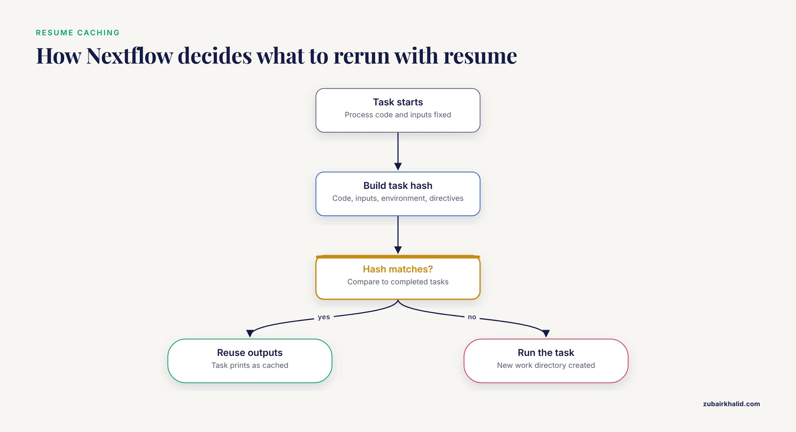
Run the same command again with -resume:
nextflow run main.nf -profile conda -resumeEvery task prints as cached:
[7a/1b2c3d] process > FASTQC (test)        [100%] 2 of 2, cached: 2 ✔
[8b/2c3d4e] process > FASTP (test)         [100%] 1 of 1, cached: 1 ✔
Nextflow computes a hash for each task from the process code, the input files and values, the software environment, and the directives. If the hash matches a completed task, the outputs are reused. Now change one thing, for example add -qualified_quality_phred 20 to the fastp command. Only fastp and everything downstream reruns, and the raw FastQC tasks stay cached. This behavior is why you never delete the work directory mid-project.
Step 9: Add Resource Monitoring
nextflow run main.nf -profile conda -resume \
    -with-report report.html \
    -with-timeline timeline.html \
    -with-trace trace.txt
trace.txt has one row per task with status, exit code, runtime, peak memory, and CPU use. It is the fastest way to diagnose a task that a scheduler killed for exceeding requested memory. The commands you will use daily:
| Command | Purpose |
|---|---|
nextflow run main.nf -profile conda | Run the pipeline |
-resume | Reuse cached tasks whose inputs and code are unchanged |
-with-report report.html | CPU and memory usage report |
-with-timeline timeline.html | Visual timeline of task start and end times |
-with-trace trace.txt | One TSV row per task |
nextflow log | List past runs with their work directories |
nextflow log <run> -f process,status,exit | Show per-task status for one run |
nextflow clean -f <run> | Delete the work directories of one run |
Step 10: From Counts to Differential Expression
Merge the per-sample featureCounts tables into one gene-by-sample matrix and hand it to DESeq2. Published Nextflow pipelines stop at exactly this handoff, because the count matrix is the interface to differential expression with DESeq2 or edgeR [4]:
library(DESeq2)

files  <- list.files("results/featurecounts",
                     pattern = "_counts\\.txt$", full.names = TRUE)
cts    <- lapply(files, function(f) read.delim(f, skip = 1, row.names = 1))
counts <- do.call(cbind, lapply(cts, function(x) x[, 6, drop = FALSE]))

coldata <- data.frame(
    condition = factor(c("control", "treated")),
    row.names = c("sampleA", "sampleB")   # must match colnames(counts) order
)

dds <- DESeqDataSetFromMatrix(countData = counts,
                              colData   = coldata,
                              design    = ~ condition)
dds <- DESeq(dds)
res <- results(dds, contrast = c("condition", "treated", "control"))
head(res[order(res$padj), ])
Feed raw counts into DESeq2, never normalized values, and give the design formula your real experimental structure. For the midstream and downstream stages (normalization, PCA, sample distance heatmaps, volcano plots, and KEGG or GO enrichment), published pipelines organize these as explicit stages after counting [8], and end-to-end differential expression pipelines have validated that this output tracks experimental measurements, with RNAflow reporting very high correlation between pipeline fold changes and qRT-PCR results [5].
Nextflow vs Snakemake
Both are excellent bioinformatics workflow managers, and the honest answer to nextflow vs snakemake is that skills transfer between them. The differences that matter in practice:
| Aspect | Nextflow | Snakemake |
|---|---|---|
| Language | Groovy-based DSL | Python-based |
| Execution model | Asynchronous dataflow channels | Directed acyclic graph of rules with file targets |
| Caching | Built-in task-hash resume | Rerun triggers based on file metadata and code changes |
| Containers and schedulers | Turnkey profiles for Docker, Apptainer, SLURM, and cloud batch | Supported through flags and profiles |
| Ecosystem | nf-core, a large collection of community-maintained pipelines | Community collections, strong in Python-heavy groups |
Choose Nextflow first if you plan to use nf-core pipelines, if your institution runs SLURM and you want scheduler submission without extra glue, or if you may move to cloud batch execution. Choose Snakemake first if your team lives in Python and thinks naturally in file targets. The pipeline you built in this tutorial maps one to one into either system, so the concepts, not the syntax, are the durable investment.
Moving to an HPC Cluster or the Cloud
The slurm profile you already wrote is most of the migration. Three practical rules:
- Launch from a persistent directory (your home or project folder), because Nextflow writes run metadata there. Put
-w /scratch/$USER/rnaseq-first/workso the work directory lands on fast shared scratch storage. - Let the config request resources per process, as the
withNameblocks do, instead of hard-coding thread counts in scripts. Tasks always usetask.cpus. - Enable Singularity or Apptainer in the cluster profile so software versions are identical on every node.
cd /home/you/rnaseq-first
nextflow run main.nf -profile slurm -w /scratch/$USER/rnaseq-first/work -resume
The same code scales far beyond a first project. The NEXT-scASV pipeline, a modular Nextflow pipeline for allele-specific variant calling from single-cell RNA-seq, processed 135,000 peripheral blood mononuclear cells from 57 donors in one week on a single node with 100 threads, which shows how far per-task parallelization carries a well-designed workflow [10]. Cloud batch executors (for example AWS Batch and Google Batch) follow the same pattern: change the profile, keep the code.
Growing Beyond Your First Pipeline
Your first pipeline is a scaffold, and the Nextflow ecosystem gives you a clear upgrade path for each limitation:
- Production bulk RNA-seq. nf-core/rnaseq is the community reference pipeline, and published laboratory pipelines build directly on it [8]. Use it once your analysis leaves the learning phase.
- Splicing and UMIs. SAMI extends the STAR-based design with unique molecular identifiers (random sequence tags that mark each original molecule so PCR duplicates can be removed) to detect splicing events that diverge from the annotation, aimed at clinical diagnostics [7].
- Alternative splicing. A systematic comparison found little overlap in splicing changes predicted by different tools and a high false-positive rate, while targets predicted by several tools validated at much higher rates, so run more than one method and trust the consensus [11].
- Long non-coding RNAs. LncPipe identifies and analyzes lncRNAs from RNA-seq data in Nextflow [12].
- Transposable elements. GeneTEFlow quantifies gene and locus-specific TE expression with Nextflow and Docker [9].
- Microbial reads in host samples. nf-rnaSeqMetagen filters host reads and characterizes the remainder with kraken2, all orchestrated by Nextflow with Singularity [3].
- Long reads. NextLongIso coordinates PacBio and ONT long-read transcript analysis, including isoform discovery and alternative splicing, in one Nextflow pipeline [13].
- Interpretation. LYNX-RNA adds large language model generated summaries on top of a Nextflow RNA-seq workflow for non-specialist audiences [14].
- Regulated settings. NNclinSSOAP packages single-cell and spatial transcriptomics with the traceability that clinical research demands, and runs from a standard laptop in about 1.5 hours [15].
Nextflow RNA-Seq Pipeline Tips
- Pin software versions from day one, with conda directives or container tags. Documented irreproducibility in RNA-seq studies is the failure mode you are preventing [5].
- Prefix every output file with the sample name, exactly as the STAR process does with
-outFileNamePrefix. - Keep all parameters in
nextflow.configand override them on the command line with-param. Code should never contain sample-specific values. - Use
-with-traceon real runs so that a failed task comes with its memory and runtime history. - Write one process per logical step. Six small processes are easier to cache, debug, and reuse than two monolithic ones.
Common Mistakes and Limitations
- Feeding gzipped FASTQ to STAR without
-readFilesCommand zcat. STAR reads the compressed bytes as text and stops almost immediately with an error about the FASTQ format. The fix is the flag shown in Step 2. - STAR index crashes on a small genome. The default
-genomeSAindexNbases 14exceeds what a small genome supports, and STAR exits with an error telling you to use min(14, log2(genome length) / 2 - 1). Compute the value, as the E. coli example in Step 5 does. - Output name collisions. If two samples write files with identical names, staging them into a downstream process aborts with an error of the form
Process 'X' input file name collision. The fix is to prefix every output with the sample identifier. - Forgetting
publishDir. Outputs exist only insidework/<hash>/<hash>/. If results seem to vanish, find them withnextflow log, which prints each task's work directory, then add thepublishDirdirective. - Hard-coded threads and memory. Scripts that ignore
task.cpusoversubscribe cluster nodes, and requests below real usage get tasks killed by the scheduler (often exit code 137). Set resources in config and verify with the trace file. - Ignoring strandedness. featureCounts counts unstranded by default. If your library is stranded, unstranded counting misassigns reads for overlapping genes. Check the forward and reverse columns of
ReadsPerGene.out.taband set featureCounts' strandness accordingly. - Mismatched mate files. If a sample has only one mate, or mates have different read counts, trimming or alignment fails for that sample.
Channel.fromFilePairswithcheckIfExists: truecatches missing files early, so keep it. - Editing files inside
work/. Manual changes are invisible to the task hash, break resume, and vanish on the next clean. Change code or config and rerun instead. - Treating the first pipeline as production-ready. It has no UMI handling, limited QC breadth, and no versioned reference management. Graduate to nf-core/rnaseq for production analyses [8] and to specialized pipelines for splicing [7] or other modalities.
- Over-trusting single-tool results. This applies beyond splicing. Computational predictions need experimental validation, and published pipelines validate their calls against measurements such as qRT-PCR for exactly this reason [5]. Plan biological replicates (three or more per group is the usual minimum) before sequencing, not after.
Frequently Asked Questions
Do I need to learn Groovy before writing a Nextflow pipeline?
No. This tutorial uses a small subset of Groovy: string interpolation, lists, and channel operators. If you can read Python or R, you can read and modify this pipeline, and you only need Groovy documentation when you add custom logic inside a process.
Can I build and test an RNA-seq pipeline on a laptop?
Yes. The local executor runs on your machine, and a smoke test with a small bacterial genome and 100,000 read pairs finishes in minutes with 16 GB of RAM. Save the human genome, which needs roughly 32 GB for the STAR index, for a bigger machine.
How does -resume decide what to rerun?
Nextflow stores a hash for every executed task based on the process code, the input files and values, the software environment, and the directives. On a rerun with -resume, any task whose hash matches a completed task is skipped and its outputs are reused.
Nextflow vs Snakemake, which should I learn first?
Learn the one your collaborators use, and both eventually. Nextflow is the stronger first choice if you want nf-core pipelines, turnkey SLURM submission, or cloud batch execution. Snakemake fits teams that prefer Python and file-target rules.
Should I use nf-core/rnaseq instead of building my own pipeline?
For production data, yes. nf-core/rnaseq implements far more QC, UMI handling, and quantification options than a first pipeline should carry. Building your own small pipeline first teaches you how those pipelines work and covers custom needs they do not.
Where do I get a genome FASTA and GTF, and which version should I pick?
Download a genome FASTA and its matching GTF from a reference database such as Ensembl or GENCODE, and always take both files from the same genome build. Record the release number in your config so every result traces to a specific reference.
How do I get from a count matrix to differential expression results?
Merge the per-sample featureCounts tables into one gene-by-sample matrix, then run DESeq2 or edgeR in R with a design formula that matches your experiment. Always provide raw counts, never normalized values, as the input.
How do I move the pipeline from my laptop to an HPC cluster?
Add a profile that sets the executor to your scheduler, for example SLURM, enables Singularity or Apptainer, and points the work directory at shared scratch storage. Then run the identical command with -profile slurm from a persistent launch directory.
Sources
- An open RNA-Seq data analysis pipeline tutorial with an example of reprocessing data from a recent Zika virus study
- SeqAcademy: an educational pipeline for RNA-Seq and ChIP-Seq analysis
- nf-rnaSeqMetagen: A nextflow metagenomics pipeline for identifying and characterizing microbial sequences from RNA-seq data
- nf-rnaSeqCount: A Nextflow pipeline for obtaining raw read counts from RNA-seq data
- RNAflow: An Effective and Simple RNA-Seq Differential Gene Expression Pipeline Using Nextflow
- TAGADA: a scalable pipeline to improve genome annotations with RNA-seq data
- Detecting unannotated splicing events in short-read RNA-seq with SAMI, a UMI-aware Nextflow pipeline
- Pipeline for RNA sequencing data analysis by combination of Nextflow and R
- GeneTEFlow: A Nextflow-based pipeline for analysing gene and transposable elements expression from RNA-Seq data
- NEXT-scASV: a Nextflow pipeline for allele-specific variant calling from single-cell RNA-seq data
- One pipeline to predict them all? On the prediction of alternative splicing from RNA-Seq data.
- LncPipe: A Nextflow-based pipeline for identification and analysis of long non-coding RNAs from RNA-Seq data.
- NextLongIso: a comprehensive Nextflow pipeline for multi-dimensional long-read RNA-seq analysis
- LYNX-RNA: A Scalable Nextflow Workflow for RNA-Seq Analysis with Integrated Large Language Models for Comprehensive Result Interpretation
- GxP-Ready Single-Cell RNA-seq and Spatial Transcriptomics End-to-End Pipeline for Clinical Research