NCBI SRA Run Selector Tutorial: Step-by-Step Guide
By Dr. Zubair Khalid, DVM, MS, PhD ·

By the end of this NCBI SRA Run Selector tutorial you will be able to find a sequencing study in the Sequence Read Archive (SRA), filter its runs by organism, library strategy, and platform, export a clean accession list, and download the underlying FASTQ files with either a browser or the SRA Toolkit on the command line. You will also know how to verify that what you downloaded matches what the authors sequenced, which is the step most people skip and later regret.
Everything here runs on free tools. For the browser-only path you need no software at all. For the command-line path you need the NCBI SRA Toolkit, which is the standard way research pipelines pull raw reads from the SRA. Published protocols routinely build their entire workflows around this download step, combining SRA Toolkit with aligners such as HISAT2, quality tools such as FastQC, and analysis in Python or R [1], and automated pipelines such as PipeSeq use SRA Toolkit as their loading step for data from the NCBI SRA database [2].
What the Run Selector Is and Where It Fits
The Sequence Read Archive is NCBI's public repository for raw high-throughput sequencing data. When researchers publish a paper based on sequencing, depositing the reads in the SRA is normally a requirement of the journal or the funder. The Run Selector is NCBI's browsing and filtering interface for one SRA study at a time. It shows every run (every individual sequencing file set) in that study as a selectable row, with sortable metadata columns and a facet sidebar for narrowing the list.
The Run Selector sits inside a wider family of NCBI databases, and understanding the relationships prevents most beginner confusion:
- SRA stores the raw reads. This is what you download when you want to run your own pipeline from FASTQ files onward.
- BioProject is the umbrella record for a study, such as a single experiment or a paper's data package.
- BioSample describes each biological sample, for example one liver tissue from one animal.
- SRA Experiment links a sample to a sequencing library, and Run is the actual unit of data, one SRR accession per file set.
- GEO (Gene Expression Omnibus) stores expression data with processed results such as count matrices, and links to the raw reads in SRA. Many transcriptomic papers cite a GEO accession for the processed data and rely on the linked SRA records for the raw reads [3].
This split matters in practice. If you want a processed expression matrix, GEO is often faster to work with. If you want to align, count, and normalize the reads yourself, you need the raw files from the SRA, and the Run Selector is the tool for choosing exactly which runs to take. Published reanalysis projects illustrate both routes. A pancreatic cancer meta-analysis pooled seven publicly available NCBI-GEO datasets with a new local cohort to find shared hub genes [4]. A machine learning study on autism spectrum disorder pulled 20 ASD and 19 typical-development RNA-seq samples from NCBI GEO and processed them with a standard R pipeline [5]. Both workflows begin the same way, with identifying and selecting the right underlying data records, and that is the job the Run Selector does for SRA.
Accession Types Explained
SRA and related NCBI records use stable accession prefixes. Each prefix tells you the level of the record, and mixing them up is one of the most common early errors.
| Prefix | Record type | Level | Typical use |
|---|---|---|---|
| PRJNA, PRJEB, PRJDB | BioProject | Study | One paper or program of work, the widest scope |
| SAMN, SAME, SAMD | BioSample | Sample | One biological specimen with attributes |
| SRX, ERX, DRX | SRA Experiment | Library | One library prepared from one sample |
| SRR, ERR, DRR | SRA Run | Data file set | The unit you actually download |
| GSE | GEO Series | Study (expression) | An expression study, links down to GSM records |
| GSM | GEO Sample | Sample (expression) | One sample in a GEO series |
A concrete example from the literature: one transcriptomic dataset of the invasive plant Thunbergia alata deposited eight transcriptomes in the SRA with BioSample accessions SAMN51331451 through SAMN51331458 [6]. Those SAMN identifiers each point to a sample record, and each sample record links to one or more SRR runs holding the sequencing data. Similarly, a single-cell RNA-seq study of kidney stone tissue lists both a GEO accession, GSE176155, and a BioProject accession, PRJNA735197, for the same data package [7]. Knowing which accession you hold tells you where to start.
The middle letters in SRA accessions encode the submitting archive. SRR records come through the standard NCBI submission path, ERR through the European archive (ENA) mirror, and DRR through the Japanese archive (DDBJ) mirror. The three archives share data, so you can work with any of them through the same NCBI tools.
Step-by-Step Walkthrough
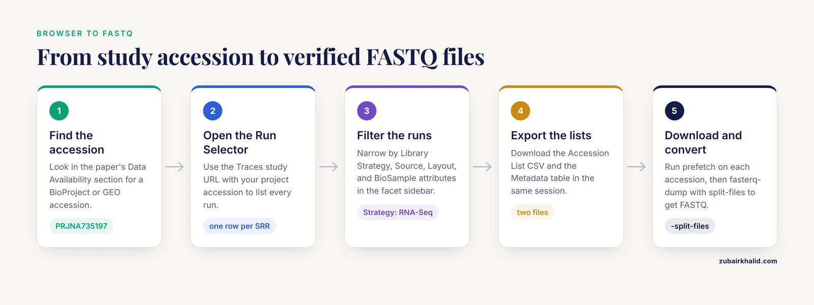
The walkthrough below covers the full path from a paper or accession number to verified FASTQ files. Steps 1 through 5 happen in the browser. Steps 6 through 8 cover downloading and verification.
Step 1. Find the study accession
Start from whatever you have. If you are reading a paper, look in the Data Availability or Data Deposition section for a phrase such as "reads are deposited under BioProject PRJNA735197" or "raw data are available at GEO accession GSE319292" [7], [3]. If you are browsing instead, go to the NCBI SRA database through the main NCBI search page, choose the SRA database from the dropdown, and search on keywords such as the organism name plus the technique, for example "Zea mays RNA-seq".
If your starting point is a GEO accession, open the GEO record and scroll to the relation links at the bottom of the page. GEO series records link explicitly to their SRA project, and clicking through lands you on the SRA side. One deposited zebrafish toxicogenomics dataset, for example, lists GEO accession GSE319292 as its home, and from there the raw reads are reachable through the linked SRA records [3].
Step 2. Open the Run Selector for the project
Every SRA study page on the NCBI website carries a "Send to" or direct link to its Run Selector. The direct URL pattern is the most reliable route:
https://www.ncbi.nlm.nih.gov/Traces/study/?acc=PRJNA735197Replace PRJNA735197 with your own project accession. This opens the Run Selector view for that BioProject, listing every run in the study. You can also paste an SRR run accession into that same URL and it will resolve to the study containing that run, which is useful when you only have a single run ID from a supplement.
Step 3. Read the columns and facets
The Run Selector page has two halves. On the right is a table of runs, one row per SRR accession. On the left is a facet sidebar that groups the runs by metadata values. The columns you will use most often are:
| Column or facet | What it tells you | Why it matters |
|---|---|---|
| Run | The SRR accession | What you will actually download |
| SampleName, BioSample | The biological sample | Lets you map runs to experimental conditions |
| Library Strategy | WGS, RNA-Seq, ChIP-Seq, amplicon, etc. | Confirms the data type matches your analysis plan |
| Library Source | Genomic, transcriptomic, metagenomic | Screens out submissions labeled differently than you expect |
| Library Layout | Paired or Single | Determines whether you expect two FASTQ files per run |
| Platform | Illumina, Ion Torrent, PacBio, ONT | Sets expectations for read length and error profile |
| AvgSpotLen | Average read length in bases | Sanity check before quality control |
| Bases, MBs | Total bases and file size | Download planning |
| Instrument | Sequencer model | Read length and quality profile expectations |
| Consent | Data use restrictions | Some human data are open, some are controlled |
Click any value in the facet sidebar, such as "Strategy: RNA-Seq", and the run table filters immediately. Clicking again clears the filter. This interaction is the core of the tool, and it is how you turn a study of 300 runs into the 6 runs you actually need.
Step 4. Filter to the runs you want
Filtering strategy depends on the study. Large consortia deposit hundreds of runs across many tissues and sequencing centers, so filter first by Strategy and Source, then by organism if the project covers several, then by sample attributes. The facet sidebar exposes the BioSample attributes the submitters provided, so in a well-annotated study you can filter directly on condition, tissue, or genotype.
Metadata quality varies enormously, and this is where reading the paper pays off. A maize RNA-seq dataset on genotype-specific responses to mycorrhizal colonization describes a fully crossed design, two inbred lines plus a hybrid under well-watered and drought conditions with and without inoculation, three biological replicates per combination [8]. If the submitters captured those factors as BioSample attributes, the Run Selector facets let you pull one treatment arm directly. If they did not, you will need the sample-to-condition mapping from the paper itself or from a supplementary table, and you should save it alongside your accession list.
Step 5. Select runs and export the accession list
Click the checkbox beside each run you want, or use the "all rows" control after filtering. Once you have a selection, three export buttons appear:
- Accession List. Downloads a plain CSV file of the selected SRR accessions, one per line. This is the file you feed to the command line in the next step.
- Metadata. Downloads the full run information table, including every metadata column, for the filtered or selected runs. Save this file in your project folder. It is the record of exactly which runs belong to which condition, and it is what you will join against your sample sheet later.
- Data Access. Shows the alternative access routes, including cloud paths, for the selected runs.
Even if you plan to download everything in the study, export the metadata table anyway. Sample annotation drifts between the paper, the BioSample records, and your memory, and the exported table is the authoritative snapshot you captured on the day you built the dataset.
Step 6. Download with the browser (small numbers of runs)
For one to a handful of runs, the browser download route works. In the SRA record page for a run, or through the Run Selector's data access links, you can fetch the .sra file directly. The catch is that a .sra file is a compressed, column-oriented archive format, not a FASTQ file. You still need SRA Toolkit to convert it, so the browser route only saves you the command-line download step, not the conversion step. For anything beyond a few runs, skip the browser and go straight to the toolkit.
Step 7. Download with SRA Toolkit
Install SRA Toolkit from NCBI's official download page for your operating system, or use the prebuilt containers. A published Colab-based protocol demonstrates the whole downstream chain, SRA Toolkit for extraction, FastQC for quality checks, Trimmomatic for trimming, HISAT2 for alignment, and feature counting, running entirely on free cloud compute [1], so the toolkit is worth installing locally even if you plan to analyze in the cloud.
First configure the toolkit so it downloads into a known location and uses your network settings:
vdb-config --interactiveIn the interactive screen, set the default output directory under the "Home" settings, enable cloud delivery if you are working on a cloud instance, and save. Non-interactive setups can use a configuration file, which matters when you script inside containers.
Now pull the runs listed in your exported accession file. The two-command pattern is prefetch followed by fasterq-dump:
mkdir -p sra_data fastq
cd sra_data

for acc in $(cat ../runs.csv | tail -n +2)
do
  prefetch "$acc"
  fasterq-dump "$acc" --split-files --threads 6 --outdir ../fastq
  gzip ../fastq/${acc}_1.fastq ../fastq/${acc}_2.fastq
done
What each command does:
prefetchdownloads the.sraarchive into your cache. It resumes interrupted downloads, which is why you run it separately rather than lettingfasterq-dumpstream over the network.fasterq-dumpconverts the archive to FASTQ.-split-fileswrites paired reads as two files, suffixed_1and_2. Without it, a paired-end run comes out as one interleaved file by default, which is the single most common beginner error in this workflow.-threads 6sets parallelism.-Osets the output directory, which we used as-outdir.tail -n +2skips the header line of the exported CSV.
For bulk project downloads, prefetch accepts a project-level accession in some tool versions, but the robust and explicit route is always the accession list you exported in Step 5. That list is also what makes the download reproducible, since anyone with the list and these commands regenerates your exact input set.
If you are testing a pipeline and want a quick preview without full downloads, use -max-size on prefetch to cap the transfer, and remember the value is in megabytes by default:
prefetch SRR000001 --max-size 200MStep 8. Verify the files
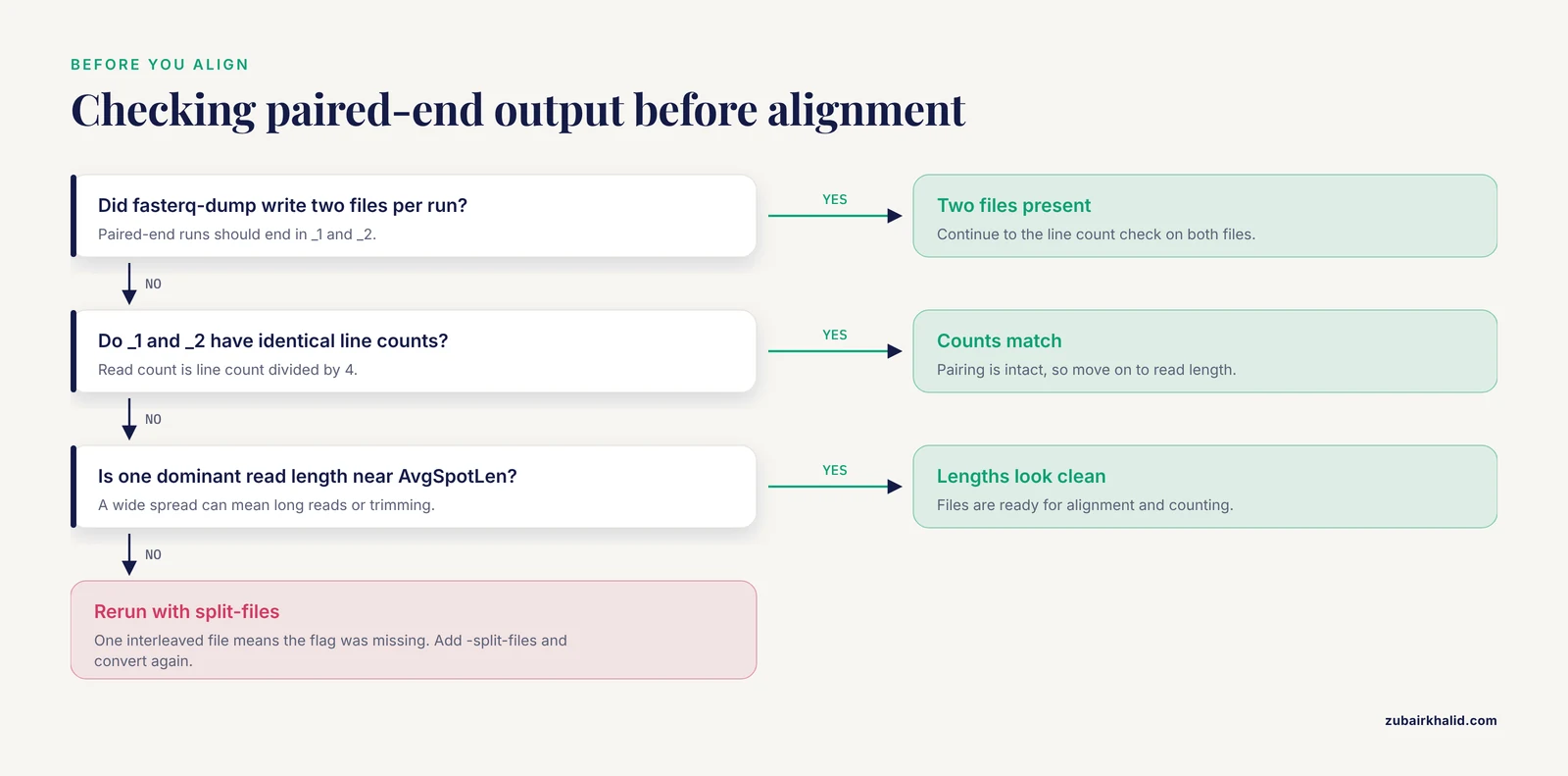
Verification has three layers. First, confirm the files exist, are paired where expected, and are plausible in size:
ls -lh ../fastq
wc -l ../fastq/SRR000001_1.fastq
A FASTQ record occupies four lines, so read count equals line count divided by 4. For a paired run, _1 and _2 must have identical line counts. This arithmetic is the fastest integrity check you have.
Second, inspect read headers and lengths:
head -n 8 ../fastq/SRR000001_1.fastq
awk 'NR%4==2{print length($0)}' ../fastq/SRR000001_1.fastq | sort | uniq -c | head
The first command shows the first two records. The second tallies read lengths. A clean run shows one dominant length close to the AvgSpotLen value you saw in the Run Selector. A wide spread can indicate variable-length reads from long-read platforms or technical trimming, either of which changes your downstream parameter choices.
Third, check the SRA metadata you downloaded in Step 5 against reality. A Bioinformatics protocol pipeline that goes from SRA download through alignment to differential expression notes that troubleshooting almost always involves handling paired-end reads correctly and resolving path and dependency issues [1]. Both problems are caught in minutes by the line-count and header checks above, and both become days of silent error if skipped.
A Worked Example Using a Published Dataset
Walk through the logic with a real study. A secondary analysis of kidney stone tissue used a publicly available single-cell RNA-seq dataset deposited under GEO accession GSE176155 and BioProject PRJNA735197, processed the raw FASTQ data through Cell Ranger version 6.0.1 aligned to GRCh38, and performed quality control, normalization, and clustering in Seurat [7]. To reproduce that analysis from scratch, the Run Selector workflow looks like this.
- Open the Run Selector at
https://www.ncbi.nlm.nih.gov/Traces/study/?acc=PRJNA735197. - In the facets, filter Library Strategy to RNA-Seq and confirm the Platform shows an Illumina instrument.
- Check Library Layout. Single-cell 10x-style data are deposited as paired-end runs, so every run should show Paired. A run showing Single here is a red flag that the submission differs from your assumption.
- Select the runs corresponding to the Randall's plaque and matched normal papilla samples, using the sample attributes or the metadata table exported from the study.
- Export the Accession List and the Metadata table.
- Download and convert with the two-command
prefetchplusfasterq-dumppattern from Step 7. - Confirm paired file counts and read lengths, then proceed to Cell Ranger.
The same skeleton transfers to bulk RNA-seq reanalyses. One workflow building a custom annotation package for Mycobacterium tuberculosis H37Rv started from a six-sample rifampicin response RNA-seq dataset, GSE292409, retrieved through NCBI [9]. Six samples means six runs or fewer, a trivial download, and the Run Selector is arguably overkill for a study that small, but the value of the tool grows exactly as study size grows. A transcriptome assembly study on maize lncRNA biology obtained its shoot and tassel RNA-seq data directly from the NCBI SRA archive and assembled transcripts for control and mutant lines [10], a classic case where selecting the right subset of runs from a larger deposited project is the difference between a clean comparison and a mixed bag.
Tips for Larger Projects
These are the tips that matter once you move from single studies to multi-study work.
Download to a cache, convert to a work directory. Keep prefetch output in one stable location and write FASTQ files to per-project folders. Re-running prefetch against a populated cache costs nothing, which makes interrupted downloads and re-conversion painless.
Mind the quality score variant. Some SRA submissions store normalized or simplified quality scores in the public copy. When you configure vdb-config, you can choose whether to prefer "lite" files with reduced quality scoring or full files with original scores. For most RNA-seq and amplicon work either is fine. For base-quality-sensitive pipelines, such as some variant callers, request the full-quality version and note the choice in your methods.
Check strand specificity before alignment. Library prep determines strand origin, and the metadata records it if the submitters filled it in. A maize dataset built with the Lexogen QuantSeq 3' mRNA-Seq kit is strand-specific and captures signal near the transcript 3' end [8]. Treating that data as standard full-transcript unstranded RNA-seq would distort read counting and alignment expectations. The Library Construction Protocol field in the run metadata often names the kit, so read it before you pick alignment parameters.
Budget disk space from the Run Selector numbers. The Bases and MBs columns let you estimate before you commit. The arithmetic is straightforward: total bases equal spots times average spot length, and the Bases column already does this for you. Double-paired data with 20 million spots and 150-base reads carry 6 billion bases of sequence, which is on the order of 6 gigabytes of uncompressed FASTQ before compression overhead. Multiply by the number of runs in your selection and confirm you have room, because a failed bulk download at 90 percent is a real thing.
Automate metadata joins, not free-text matching. Join your exported Run Selector metadata table to your experimental design table on the run accession, which is a stable key. Matching on sample names typed into spreadsheets is where silent sample swaps happen.
Reproducibility is the point. Several recent pipelines emphasize reproducibility as a design goal, with PipeSeq wrapping SRA Toolkit loading, HISAT2 alignment, StringTie assembly, FeatureCounts counting, and DESeq2 statistics behind a single interface [2]. Whatever your pipeline looks like, the SRA accession list, the metadata export, the toolkit version, and the conversion commands are the four pieces that make your raw-data provenance auditable. Record all four.
Common Mistakes and Limitations
Confusing GEO and SRA accessions. A GEO series accession like GSE292409 points to expression data and processed files [9], while the raw reads live in SRA records reached through the linked project. Searching an SRA tool for a GSE accession either fails or silently returns nothing useful. Resolve the accession to its BioProject first, then open the Run Selector.
Expecting paired-end splitting by default. fasterq-dump without -split-files writes one file. If your downstream tools assume two files and you feed them the interleaved single file, alignment fails or, worse, produces plausible-looking nonsense. The line-count check from Step 8 catches this immediately, since the interleaved file will have twice the lines of the _1 file you expected.
Assuming SRA files are identical to the sequencer output. The SRA stores what the submitter deposited, which may be processed relative to the raw instrument output. Bases may be normalized and quality scores may be simplified. If your methods section claims you analyzed "raw" data, verify what you actually received, because the distinction occasionally matters for quality-controlled analyses.
Ignoring Library Strategy. Filtering by Strategy takes one click and prevents the classic error of building a transcriptome pipeline around a run that is actually whole-genome sequencing. Cross-check the Strategy facet against the paper's description before selecting.
Downloading before checking size and consent. The MBs column and the Consent facet exist for a reason. Human data can be open-access or controlled-access, and controlled data require authorized access through dbGaP or an equivalent mechanism rather than a simple download. Check the Consent column before planning a download, not after.
Losing the metadata linkage. Runs alone are useless. Without the mapping from SRR accession to biological condition, your downloaded FASTQ files cannot be analyzed as a designed experiment. Export the metadata table in the same session in which you export the accession list, because submitter records are occasionally revised later.
Assuming quality is uniform across a study. Even within one BioProject, runs may come from different instruments, flow cells, or read length settings. The AvgSpotLen and Instrument columns in the Run Selector table expose that heterogeneity before it surprises you mid-pipeline.
One limitation applies to any reanalysis of public data. Deposited metadata is only as complete as the submitters made it, and the paper remains the ground truth for experimental design. Where the Run Selector facets and the paper disagree, stop and resolve the discrepancy before analyzing anything, and remember that individual datasets can have quirks that no tutorial anticipates.
Frequently Asked Questions
What is the difference between the SRA, GEO, and the Run Selector?
The SRA stores raw sequencing reads, GEO stores expression data with processed results such as count matrices, and the Run Selector is NCBI's browser interface for filtering and selecting runs within one SRA study. Use GEO when you want processed data, use the Run Selector when you want to pick and download raw reads.
How do I download FASTQ files from the SRA Run Selector?
Export the Accession List from the Run Selector, then run prefetch on each accession followed by fasterq-dump, split-files from the SRA Toolkit. The browser can download .sra files directly, but you still need the toolkit to convert them to FASTQ.
What do the SRR, SRX, SRP, and SAMN prefixes mean?
SRP is a study, SAMN is a biological sample, SRX is a sequencing library, and SRR is an individual run or data file set. You download SRR accessions and use the higher-level accessions to organize and interpret them.
Why did fasterq-dump give me one FASTQ file instead of two for paired-end data?
By default fasterq-dump writes a single interleaved file for paired-end runs. Add the -split-files flag to produce separate _1 and _2 files, and confirm equal line counts in both.
How do I download all runs in a BioProject at once?
Filter or select the runs in the Run Selector, export the Accession List CSV, and loop over it with prefetch and fasterq-dump in a shell script. Check the MBs column first to confirm the total download size fits your storage.
Can I use the Run Selector without installing anything?
Yes. Filtering, selecting, and exporting accession lists and metadata tables all happen in the browser with no software installed. You only need SRA Toolkit once you want FASTQ files on disk.
How large are SRA datasets and how much disk space do I need?
The Bases and MBs columns in the Run Selector give exact totals per run before you commit. As a rule of thumb, a paired-end run with 20 million reads of 150 bases carries about 6 billion bases, roughly 6 gigabytes of uncompressed FASTQ, so multiply those figures by your run count.
Why is my downloaded SRA file not a FASTQ file?
SRA files use NCBI's own compressed archive format, not FASTQ. Run fasterq-dump on the downloaded file to convert it, or use prefetch plus fasterq-dump together so the download and conversion happen as separate, resumable steps.
Sources
- Streamline Protocol for Bulk-RNA Sequencing: From Data Extraction to Expression Analysis.
- Development and validation of the PipeSeq program for RNA-seq data analysis in the Chlamydomonas reinhardtii as a model.
- Transcriptomic data of larval zebrafish exposed to environmentally relevant levels of uranyl nitrate and sodium arsenite.
- Dysregulated expression of cell cycle regulators CDC20, PLK1, BUB1, CDC45, CDCA5 in pancreatic ductal adenocarcinoma.
- Identification of Potential Biomarkers in ASD Integrating RNA Seq Data and Machine Learning Approaches.
- Transcriptomic dataset of the invasive species Thunbergia alata and its congener Thunbergia grandiflora (Acanthaceae) in Cali, Colombia.
- Expression analysis of epithelial membrane protein 1 (EMP1) gene in kidney stone patients.
- Illumina RNA-seq data of Genotype-specific responses of maize plants to Funneliformis mosseae.
- Enhanced RNA-Seq Expression Profiling and Functional Enrichment in Non-model Organisms Using Custom Annotations.
- Computational prediction of the interaction network between long non-coding RNAs and microRNAs in maize based on the transcriptome of the fuzzy tassel mutant line.