NCBI Pathogen Detection Pipeline
By Dr. Zubair Khalid, DVM, MS, PhD ·

By the end of this guide you will be able to search the NCBI Pathogen Detection Isolates Browser, download isolate metadata and antimicrobial resistance calls in bulk, run the same resistance-detection software that NCBI uses on your own assemblies, interpret SNP cluster results without overreading them, and deposit your own sequenced isolates so they appear in the system. You will need a modern web browser, a Mac or Linux shell with curl and wget, Python 3, and, for the local analysis steps, the NCBI datasets command-line tool and NCBI AMRFinderPlus. All of these are free, and every command below runs on a standard laptop.
What the NCBI Pathogen Detection Pipeline Is
The NCBI Pathogen Detection Pipeline is a public surveillance system built and maintained by the National Center for Biotechnology Information (NCBI). Its public face is the Pathogen Detection Isolates Browser (PDIB), a web interface where bacterial pathogen isolates from food, clinical, environmental, and veterinary sources are collected, analyzed, and clustered so that public health and food safety laboratories can find genetically related isolates within minutes instead of weeks.
The data flowing through it come largely from two large sequencing networks. The FDA's GenomeTrakr network sequences food and environmental isolates, and the CDC's PulseNet sequences clinical isolates. Academic and industry laboratories contribute as well. The NCBI Pathogen Detection database collections have grown through exactly this coordination and technology sharing, and published work built on the resource describes analysis of roughly 160,000 sequenced isolates spanning organisms such as Salmonella enterica and Listeria monocytogenes [1].
Three things make the pipeline unusual among surveillance systems:
- It is automatic. Once an isolate's reads and metadata are submitted, NCBI assembles the genome, calls antimicrobial resistance determinants, computes a SNP tree against a reference, and places the isolate into a SNP cluster without any analyst in the loop.
- It is public. Any user can search, browse, and download the same outputs the submitters see, which is why the resource supports not only outbreak investigation but also food safety risk research and method development [1].
- It is standardized. Every isolate is analyzed with the same versions of the same tools, which makes a SNP cluster in the browser directly comparable across laboratories.
This matters because molecular epidemiology has become a core tool for diagnosing disease and tracing infection routes, and platforms that combine shared sequence information with standardized analysis are increasingly the backbone of that work [2]. A pathogen-specific database with an integrated typing module, such as the European classical swine fever database, pioneered this model on a smaller scale [2]. NCBI extended it to many organisms at national scale.
How a Genome Moves Through the Pipeline
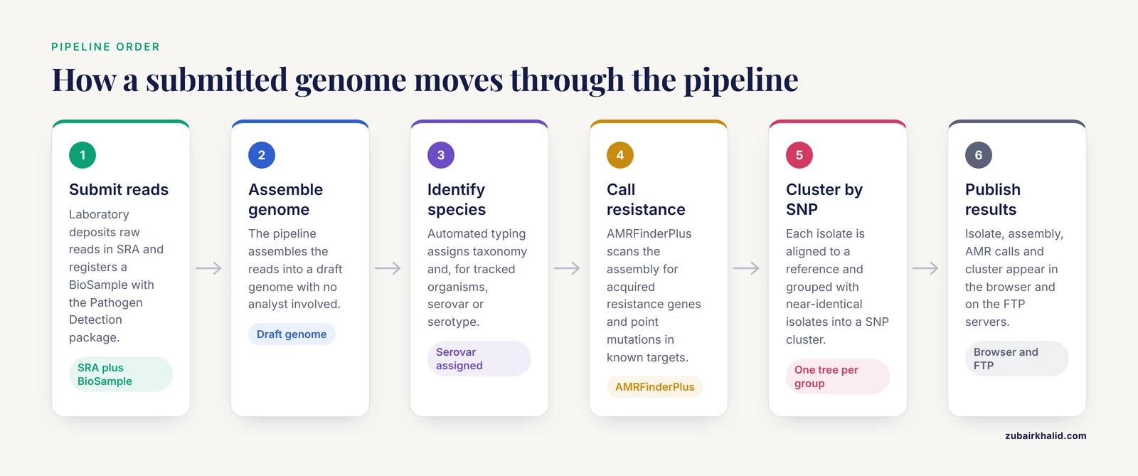
Understanding the flow helps you interpret everything you download later. The steps, in order, are:
- Submission. A laboratory deposits raw sequence reads in the Sequence Read Archive (SRA) and registers a BioSample record using the Pathogen Detection package. That package enforces the attribute fields the pipeline needs, such as organism, strain, isolation source, collection date, and geographic location.
- Assembly. The pipeline assembles reads into a draft genome.
- Species and serovar identification. Automated typing assigns taxonomy and, for tracked organisms, serovar or serotype.
- Antimicrobial resistance detection. NCBI AMRFinderPlus scans the assembly and predicted proteins for acquired resistance genes, point mutations in known targets, and other resistance determinants.
- SNP clustering. The pipeline aligns each isolate against a reference, calls single nucleotide polymorphisms (SNPs), and groups isolates that differ by very small numbers of SNPs into clusters, one tree per tracked organism or serovar group.
- Publication. The isolate, its assembly, its AMR calls, and its cluster assignment appear in the Isolates Browser, and the underlying files are released to NCBI's FTP servers for bulk download.
If you are new to how the underlying databases fit together, the pipeline sits on top of several you should know as part of any guide to how to use NCBI: SRA holds the raw reads, BioSample holds the biological and epidemiological attributes, Assembly holds the contig sets, RefSeq holds curated reference genomes, Taxonomy holds the naming, and the NCBI Virus database holds viral sequences in a search-friendly form [3]. RefSeq genomes are also the substrate for benchmarking new analysis methods, which is how the broader community validates the reference base the pipeline depends on [4].
NCBI's platform goes beyond storage. Reviews of its protein analysis capabilities describe how the same ecosystem supports phylogenetic comparison and functional prediction once sequences are in hand [5], and sequence-based searches on NCBI are routinely the first step in building templates for structural work [6]. The Pathogen Detection pipeline is best understood as one specialized application of that ecosystem rather than a stand-alone site.
NCBI Pathogen Detection Pipeline Step by Step
This walkthrough uses Salmonella enterica as the worked example because it is the organism with the most developed downstream literature. Every step generalizes to the other tracked bacteria.
Step 1. Orient yourself in the Isolates Browser
Open https://www.ncbi.nlm.nih.gov/pathogens/. The page opens on a tabbed browser with one tab per tracked organism group, such as Salmonella, Escherichia coli/Shigella, Listeria, and Campylobacter. The table lists one row per isolate, with columns for the isolate name, strain, serovar, isolation source, geographic location, collection date, assembly accession, AMR markers found, and the SNP cluster it belongs to.
Practice this search:
- Type
Enteritidisin the search box on the Salmonella tab to see isolates of that serovar. - Use the filters on the left to restrict to a specific state or country and a collection date range.
- Click any isolate name to open its detail page, which links the BioSample, the SRA run, the assembly, and the AMR results.
Note the "Download" button. It exports the exact filtered table you are viewing as a CSV, including the SNP cluster identifiers. This is the fastest way to pull a small working set, and it is how most people should start.
Step 2. Take a snapshot of the browser table
Before doing anything else, save your filtered view.
# Save the CSV you downloaded from the browser button
mv Salmonella_Enteritidis_2020-2025.csv snapshot_2026-11-11.csv

# Check the columns you actually received
head -1 snapshot_2026-11-11.csv
wc -l snapshot_2026-11-11.csv
Expected output is a header line listing the field names and a line count matching the number of isolates in your filtered view, for example 1,432 rows. Keep this file immutable. The browser changes every day as new submissions are processed, so any reproducible analysis needs a dated snapshot, not a live query.
Step 3. Bulk download from the NCBI FTP servers
For anything larger than a few thousand isolates, use the bulk files. NCBI publishes the pipeline's raw outputs, including metadata tables, AMR results, pangenome protein sets, and reference genome lists, under the pathogen/Results tree on its FTP server. File names carry a build number that changes with each daily release, so always list the directory first rather than hardcoding a file name from a tutorial.
# List the current build files for Salmonella
curl -s "https://ftp.ncbi.nlm.nih.gov/pathogen/Results/Salmonella/" \
  | sed -e 's/href=//g' -e 's/"//g' | grep -i metadata
Expected output is one or more file names, for example a line containing Salmonella.metadata and a build suffix. Then download the current file and its AMR companion:
# Copy the actual current names from the listing above
BASE="https://ftp.ncbi.nlm.nih.gov/pathogen/Results/Salmonella"
wget "$BASE/Salmonella.metadata.tsv.gz" -O salmonella_metadata_build-current.tsv.gz
gunzip salmonella_metadata_build-current.tsv.gz

# Inspect the header before parsing anything
head -1 salmonella_metadata_build-current.tsv
Expected output is a tab-separated header with fields identifying the isolate, its BioSample and assembly accessions, serovar, source, geography, collection date, and SNP cluster membership. Column names have been stable in practice but are not contractual, so code that parses them should read the header first.
Step 4. Parse the metadata with Python
A short script turns the metadata table into a working list.
import csv

with open("salmonella_metadata_build-current.tsv") as handle:
    reader = csv.DictReader(handle, delimiter="\t")
    rows = list(reader)

print("total isolates:", len(rows))

# Keep isolates collected in 2024 from one serovar, adjusting
# the field names to match the header you printed in step 3
kept = [
    r for r in rows
    if r["serovar"] == "Enteritidis"
    and r["collection-date"].startswith("2024")
]
print("kept isolates:", len(kept))

for r in kept[:3]:
    print(r["isolate"], r["geo-loc-name"], r["SNP-cluster"])
Expected output is a count of total isolates, a smaller count of kept isolates, and three example lines such as:
total isolates: 412537
kept isolates: 8941
FSIS22015789  United-States:KS  PA7
FSIS22016102  United-States:IA  PA7
CVM_NARMS-Sal-2773  United-States:MN  PA12
The exact numbers will differ because the dataset grows daily. What should match is the shape, one row per isolate with location and cluster fields populated.
Step 5. Run AMRFinderPlus on your own assembly
The pipeline calls resistance determinants with NCBI AMRFinderPlus, which is freely available and installs on Linux and macOS. Running it locally on your own isolate lets you reproduce the browser's calls for your samples before they appear there.
# Update the AMRFinderPlus databases to the current release
amrfinder -u

# Run against a draft assembly in nucleotide FASTA form,
# specifying the organism so point mutations are also evaluated
amrfinder -n GCA_012345675.1_genomic.fna \
          -O Salmonella \
          -o amr_results.tsv

# View the calls
column -t -s $'\t' amr_results.tsv | head -12
Expected output is a tab-separated table. An abridged view of the format looks like this, with values shown only as an example of the structure:
Protein identifier   Contig id    Start  Stop   Orientation  Element symbol   Element type  Class            Subclass
KKAHHAHH_00421       contig00012  4411   5652   +            blaTEM-1         AMR           PENICILLIN       PENICILLIN
KKAHHAHH_00577       contig00014  9122   9974   -            tet(A)           AMR           TETRACYCLINE     TETRACYCLINE
gyrA_p.S83Y          contig00002  19544  19717  +            gyrA_S83Y        AMR           FLUOROQUINOLONE  FLUOROQUINOLONE
The columns that matter most are the element symbol, the class and subclass, and the method column, which distinguishes a perfect or exact match from a partial one. A partial coverage value on a resistance gene usually means a truncated gene at a contig edge, which is a draft assembly artifact and a common reason a call differs between runs. Compare your calls for any isolate that already exists in the browser by opening that isolate's page and checking its AMR marker list against amr_results.tsv.
Step 6. Work with SNP clusters
SNP clusters are the heart of the system. Isolates that align against a shared reference and differ by very small SNP distances are placed in the same cluster, and the cluster is the unit you will investigate when you suspect a common source.
The browser gives you the cluster membership, but careful work goes further. A recent comparative protocol examined 354 Salmonella isolates spanning 59 SNP clusters and 21 serotypes identified in the Isolates Browser across beef, chicken, pork, and turkey commodities [7]. The authors combined two analyses. The first was a core chromosome SNP analysis, restricted to the conserved chromosome, which agreed closely with the PDIB results. The second was a variable genome analysis that brought in nearest-neighbor complete closed reference genomes and looked beyond the core chromosome. That second analysis uncovered additional differences, including large deletions, prophages, and plasmid variability, that the PDIB SNP analysis did not detect, and in outbreak case studies involving serotypes Newport and Hadar these features helped distinguish closely related isolates [7].
The practical procedure that follows from this work:
- Download your SNP cluster's isolates from the browser snapshot.
- Fetch complete, closed genomes of the nearest neighbors from RefSeq using the
datasetscommand-line tool. - Run a core genome SNP analysis to confirm the PDIB relationship.
- Add a variable genome comparison for prophages, plasmids, and large deletions before declaring two isolates identical.
# Fetch complete RefSeq genomes for the nearest-neighbor analysis
datasets download genome taxon "Salmonella enterica" \
  --assembly-level complete \
  --include genome

unzip ncbi_dataset.zip
ls ncbi_dataset/data/GCF*/
Expected output is a directory tree containing one genomic FASTA per downloaded assembly. Feed the corresponding closed reference into your SNP pipeline alongside your cluster's draft assemblies so that the core chromosome analysis and the plasmid and prophage comparison both have a stable anchor.
For the plasmid side, established workflows pair AMRFinderPlus gene calls with plasmid characterization tools such as MOB-suite, and real-time plasmid transmission systems have combined Mash distance searches for plasmid sharing with core genome typing for clonal relatedness in surveillance settings [8]. You do not need that full apparatus for a single question, but if your cluster spans multiple food commodities, checking whether the same resistance plasmid appears on different backbones is often the most informative test you can run.
Step 7. Submit your own isolates
To get your isolates into the system, complete three deposits in order:
- SRA. Upload the raw reads with a submission account, including sequencing platform and library details.
- BioSample. Register each isolate using the Pathogen Detection package and fill in every required attribute, most notably organism, strain, serovar where known, isolation source, isolation host, collection date, and geographic location at the state or province level.
- Link and release. Link the BioSample to the SRA reads, release the records, and let the pipeline process them. The isolate typically appears in the browser after the next processing cycle for that organism.
The Pathogen Detection package exists precisely because the automated pipeline cannot guess your metadata. An isolate submitted with an empty collection date or a vague geographic field still gets analyzed, but it loses the epidemiological context that makes it findable and interpretable, which defeats the purpose for everyone downstream.
Step 8. Verify that what you downloaded is what you think it is
Three checks catch most problems:
- Accession round trip. Pick five BioSample accessions from your file and paste them into the NCBI search box. Each should resolve to the correct isolate with matching serovar and geography.
- Local reproducibility. Rerun AMRFinderPlus locally on one assembly you downloaded from the browser and compare gene calls with the isolate's web page. Small differences usually mean a database version mismatch, so check which version your local tool reports.
- Date sanity. Sort your snapshot by collection date and confirm the minimum and maximum dates parse correctly. Unparsed dates silently drop isolates from time filters later.
Key Files and Options at a Glance
| Resource | Where it lives | What it gives you | Typical use |
|---|---|---|---|
| , - | , - | , - | , - |
| Isolates Browser | ncbi.nlm.nih.gov/pathogens/ | Searchable isolate table with clusters and AMR markers | Interactive exploration, small exports |
| Browser CSV download | Download button on filtered view | The exact filtered table | Quick snapshots, case reviews |
| Bulk metadata table | FTP pathogen/Results tree | One row per isolate for the whole organism | Large-scale studies, dashboards |
| AMR results files | FTP pathogen/Results tree | Gene and point mutation calls per isolate | Resistance surveillance, method comparison |
| Reference genome lists | FTP pathogen/Results tree | The references the pipeline used | Reproducing SNP analyses locally |
| AMRFinderPlus | Local install | Same resistance calls as the pipeline | Pre-submission checking, own isolates |
datasets CLI | Local install | RefSeq genome packages by taxonomy and assembly level | Building reference sets for cluster work |
| SRA and BioSample | ncbi.nlm.nih.gov/sra, /biosample | Raw reads and isolate attributes | Submission and provenance |
How to Use NCBI Effectively Around This Pipeline
The Pathogen Detection system is one node in a much larger network. The International Nucleotide Sequence Database Collaboration, which links NCBI's GenBank with its partner databases, holds the enormous base of nucleotide and protein sequences that makes any surveillance pipeline possible, and virus-specific databases have grown up alongside the general ones to add curated content and specialized features [9]. Knowing which node to query for which question is most of the skill.
- For viruses, the pipeline is not the primary tool. The NCBI Virus database supports targeted sequence retrieval and comparison, and studies of coronavirus spike protein evolution have drawn spike and receptor sequences directly from it for structural analysis [3]. Pathogen-specific resources such as the Virus Pathogen Resource (ViPR) provide curated virus databases with integrated analysis tools for organisms like hepatitis C [10], and specialized alignment approaches such as EvoPrinter can superimpose hundreds of pairwise alignments to compare large numbers of flavivirus or filovirus genomes for shared or unique identity SNPs [11]. For phylogeographic and molecular dating work on viral sequences, integrated toolkits such as VirPhyKit bundle sequence curation, spatiotemporal subsampling, and migration analysis into one interface [12].
- For metagenomic samples, use a metagenomic pipeline. The Pathogen Detection pipeline is built for cultured isolates of tracked bacteria, not for unbiased metagenomic next-generation sequencing. Cloud-based systems fill that role. IDseq accepts raw metagenomic data, performs host and quality filtration, then runs an assembly-based alignment pipeline that assigns reads and contigs to taxonomic categories, with background models and spike-in control recognition designed for detecting novel pathogens [13]. Pathosphere offers a similar cloud-hosted, open-source model for uploading data and running detection pipelines without local hardware [14]. Independent evaluation of three such pipelines, CZ ID, Genome Detective, and Galaxy, on shotgun metagenomic data from Aedes mosquitoes found that CZ ID and Genome Detective performed well for detection accuracy, with validation against both a mock virus database and publicly available NCBI SRA datasets [15].
- For protein questions about the organisms you find. Once the pipeline points you to an organism or a plasmid, NCBI's protein repositories and analysis services support downstream work such as phylogenetic characterization and function or structure prediction [5], and NCBI sequence searches routinely serve as the template discovery step for structural modeling projects [6].
- For reference genomes and method benchmarking. RefSeq remains the standard substrate. Simulated viral metagenomic communities built from RefSeq genomes were used to compare assemblers such as Newbler, Celera, Minimo, Velvet, MetaVelvet, and Genovo on assembly length, read recruitment, and accuracy, a reminder that the reference database's content shapes what any downstream tool can detect [4].
Tips for Getting Reliable Results
- Filter in two passes. First restrict by serovar or species and geography, then narrow by collection date. A single broad search on a busy organism returns more rows than the browser will happily export, and the two-pass approach keeps each view under the export limits.
- Always snapshot. Daily builds change cluster assignments and metadata. Date-stamp every file you download and record the build identifier from the FTP listing in your analysis notes.
- Check the method column in AMR output. A gene reported with partial reference coverage is a weaker claim than an exact match. When a call matters, for example a carbapenemase in a clinical isolate, verify coverage and identity numbers rather than taking the symbol alone.
- Use closed genomes as anchors for cluster work. The comparative protocol work on Salmonella SNP clusters showed that including nearest-neighbor complete closed reference genomes in the evaluation improved resolution of genetic relatedness among isolates, because closed references give the assembly a stable backbone [7].
- Pair gene calls with plasmid context when resistance repeats across unrelated isolates. Characterizing the plasmid, not just the gene, distinguishes clonal spread from horizontal plasmid transfer, which is the pattern most worth flagging in a surveillance setting [8].
- Document your search terms and filter state. The browser does not give you a permanent URL for every filter combination in the same way a database query does, so write down exactly what you clicked.
- Treat the browser as the index, the FTP as the data. Interactive pages are for questions you ask once. Everything you plan to compute on belongs in a local file from the bulk downloads.
Common Mistakes and Limitations
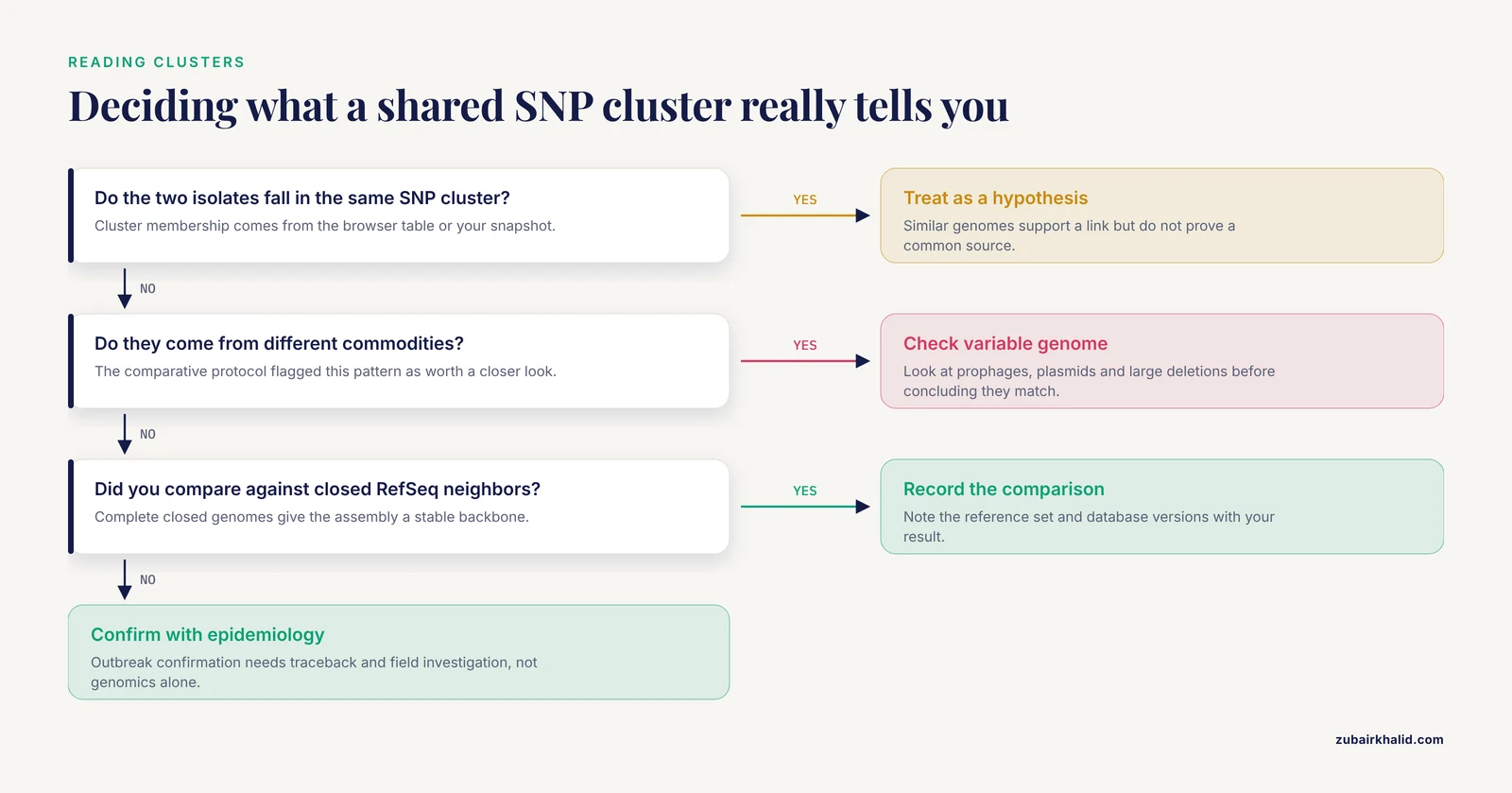
- Reading a SNP cluster as proof of a common source. A cluster is a genomic observation. Outbreak confirmation needs epidemiological investigation and traceback, and the genomic result is one line of evidence among several. Overstating it is the single most common misuse of the resource.
- Stopping at the core chromosome SNP result. The PDIB relies on SNP analysis of draft genomes, and that reliance can obscure real genetic differences. The comparative Salmonella protocol found large deletions, prophage differences, and plasmid variability within SNP clusters that the browser's own analysis did not surface [7]. If two isolates sit in the same cluster but come from different commodities, look at the variable genome before concluding they are the same strain.
- Trusting metadata you did not curate. High-quality genomic data in the system is not always coupled to high-quality epidemiological or food chain metadata, and the curation burden falls on the analyst for any study built on the resource [1]. Location, source, and date fields vary in completeness among submitters.
- Hardcoding FTP file names. Build numbers change with every release and a script written against last month's file name fails silently or downloads nothing. Always list the directory inside your script.
- Expecting the pipeline to handle metagenomes or novel agents. Detection methods that depend on homology to previously annotated sequences in NCBI databases can miss organisms with limited similarity to anything annotated, a limitation documented directly in cloud pipeline testing on spiked samples [14]. Experimental work has also shown that isolation methods recover viruses that metagenomic sequencing misses, including phages with no close relative among millions of genomes in NCBI and IMG/VR datasets, and that roughly half of NCBI-deposited virus isolates are detectable in the corresponding uncultured virus database, meaning low-abundance or unusual viruses are underrepresented in sequence-based views [16]. Metagenomic surveillance needs dedicated pipelines such as IDseq or CZ ID, not the isolate browser [13] [15].
- Confusing resistance gene presence with resistance phenotype. AMRFinderPlus reports detected genes, known point mutations, and their classes. It does not report a minimum inhibitory concentration, and gene presence does not always translate to phenotypic resistance. Susceptibility testing remains the phenotype of record.
- Comparing results across database versions. AMRFinderPlus database updates change calls. Note the database version with every result, yours and the browser's.
- Submitting incomplete BioSample records. Missing required attributes in the Pathogen Detection package weakens the isolate's findability and its value to every downstream cluster analysis. Fill in the geographic and source fields with the most specific standard values available.
- Assuming absence in the browser means absence in nature. The system tracks a defined set of organisms and draws from participating submitter networks. Organisms outside the tracked set, isolates from regions without active submission, and strains never sequenced will not appear, and negative searches need that caveat attached.
Frequently Asked Questions
What is the NCBI Pathogen Detection Pipeline?
It is a public surveillance system that collects bacterial pathogen genome sequences from contributing laboratories, analyzes each isolate automatically for assembly, antimicrobial resistance determinants, and SNP-based relatedness, and presents the results in the Isolates Browser with bulk data downloads on NCBI's FTP servers.
How do I find isolates from a specific outbreak or food source?
Use the Isolates Browser's search box together with the left-side filters for serovar, isolation source, geography, and collection date, then export the filtered table with the Download button. Isolates in the same SNP cluster are the candidates for common-source investigation, pending epidemiological confirmation.
Is the data free to download and use?
Yes. The Isolates Browser, the SRA reads, the assemblies, and the bulk FTP files including metadata and AMR results are publicly available at no cost, which is what makes the resource usable for both public health response and independent research [1].
Does the pipeline analyze metagenomic samples or viruses?
No. The pipeline is designed for cultured bacterial isolates of tracked organisms. Metagenomic samples need dedicated metagenomic pipelines such as IDseq or CZ ID [13] [15], and viral sequence work is better served by the NCBI Virus database and virus-specific resources [3] [10].
How do I submit my own isolates to the system?
Deposit raw reads in SRA, register each isolate as a BioSample using the Pathogen Detection package with all required attributes filled in, link the records, and release them. The pipeline then processes the isolate automatically and it appears in the browser.
How current is the data in the Isolates Browser?
The system processes submissions continuously and the bulk files are rebuilt on a daily release cycle, so new isolates appear regularly. Because the data change every day, save a dated snapshot of any filtered table before you analyze it.
Does matching SNP clusters mean two isolates came from the same source?
No. A SNP cluster means the genomes are extremely similar, which supports but does not prove epidemiological linkage, and variable genome features such as prophages and plasmids can distinguish isolates that share a cluster [7]. Treat cluster membership as a hypothesis for traceback and field investigation.
Can I reproduce the pipeline's analysis on my own computer?
Substantially, yes. AMRFinderPlus is the same resistance-detection software the pipeline uses and runs locally against your assemblies with the amrfinder -n command [8]. Full SNP tree reproduction requires the reference genomes the pipeline used, which NCBI publishes on its FTP servers, plus your own alignment and clustering step.
Sources
- GenomeGraphR: A user-friendly open-source web application for foodborne pathogen whole genome sequencing data integration, analysis, and visualization
- The European Classical Swine Fever Virus Database: Blueprint for a Pathogen-Specific Sequence Database with Integrated Sequence Analysis Tools
- COVID-19 Pathogen Viral Evolution Leading to Increased Infectivity
- Comparison of different assembly and annotation tools on analysis of simulated viral metagenomic communities in the gut
- Protein analysis capabilities in the NCBI bioinformation system
- Comparison, Analysis, and Molecular Dynamics Simulations of Structures of a Viral Protein Modeled Using Various Computational Tools
- A Computational Protocol for Enhanced Characterization of Sequence Differences Among Salmonella enterica isolates within SNP Clusters Identified in the NCBI Pathogen Detection System.
- Real-time plasmid transmission detection pipeline.
- Bioinformatics Goes Viral: I. Databases, Phylogenetics and Phylodynamics Tools for Boosting Virus Research
- Hepatitis C Virus Database and Bioinformatics Analysis Tools in the Virus Pathogen Resource (ViPR).
- Flavivirus and Filovirus EvoPrinters: New alignment tools for the comparative analysis of viral evolution
- VirPhyKit: An Integrated Toolkit for Viral Phylogeographic Analysis
- IDseq-An open source cloud-based pipeline and analysis service for metagenomic pathogen detection and monitoring
- Pathosphere.org: pathogen detection and characterization through a web-based, open source informatics platform.
- Exploration of viral diversity in Aedes mosquitoes employing different shotgun metagenomic data analysis pipelines.
- Identification and Genomic Analysis of a New Viral Species With Low Similarity to Existing Viruses.