NCBI Gene Expression Section RNA-seq: Step-by-Step Guide
By Dr. Zubair Khalid, DVM, MS, PhD ·

By the end of this guide you will be able to take any public RNA-seq dataset from the gene expression holdings of NCBI, download the raw reads, run quality control, align them to a reference genome, count reads per gene, test for differential expression with DESeq2, and run functional enrichment, using only free and open-source tools. You will also know the failure points that ruin most first attempts, from mismatched accession types to wrong strandedness settings.
Everything here runs on a laptop with 16 GB of RAM if you analyze a few samples, or in a free Google Colab session if you have no local hardware at all, which is the approach used by a published start-to-finish protocol built around SRA Toolkit, FastQC, Trimmomatic, HISAT2, Samtools, and Subread [1]. Basic command-line familiarity helps, but every command is written out in full.
How NCBI Stores Gene Expression Data
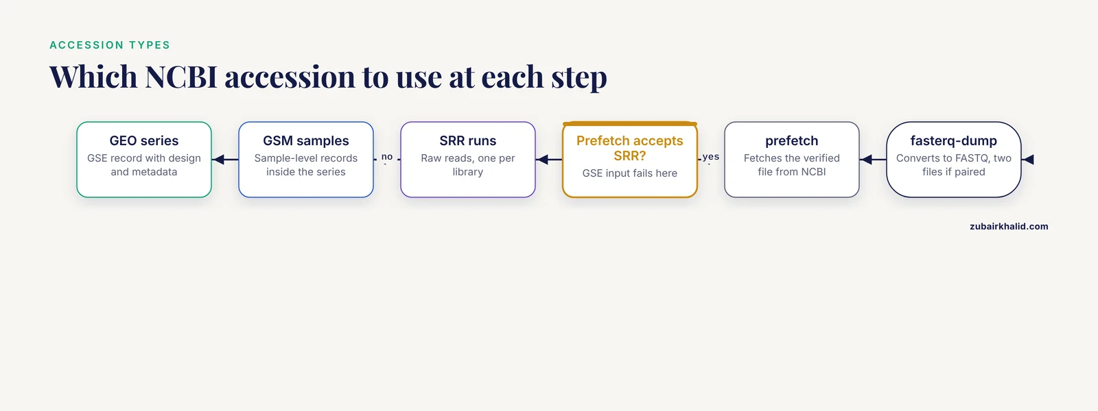
Before you touch a terminal, you need to understand how NCBI organizes expression data, because nearly every beginner problem in this workflow traces back to confusing one accession type with another. This short tour doubles as a practical entry to the wider NCBI databases guide, since the same accession logic applies across resources.
NCBI archives raw expression data in two connected resources:
- GEO (Gene Expression Omnibus) holds the study-level record, the sample metadata, and usually a matrix of processed values such as normalized counts. A series accession looks like GSE292409, the Mycobacterium tuberculosis rifampicin-response dataset used to demonstrate custom annotation workflows [2]. Individual samples inside a series carry GSM numbers, for example GSM followed by five digits.
- SRA (Sequence Read Archive) holds the raw sequencing reads, the FASTQ files you actually want for a full pipeline. A run accession looks like SRR followed by seven to nine digits. Many GEO series, including the larval zebrafish contaminant-exposure dataset GSE319292, link directly from the GEO page to the underlying SRA runs [3].
A third identifier, the BioProject accession (formatted PRJNA plus digits), ties everything together at the study level. The kidney stone single-cell dataset GSE176155, for example, is registered under BioProject PRJNA735197, and both accessions appear on the same NCBI landing pages [4].
The practical rule is simple. Use GEO to evaluate whether a study is worth your time, because GEO carries the design, the metadata, and the processed matrices. Use SRA to pull raw reads when you want to run your own pipeline from scratch. Published reanalyses almost always start at GEO and end at SRA: researchers mining the NCBI GEO public database for bulk RNA-seq followed exactly this path when they assessed cell-type composition in baboon kidney cortex samples [5], and a pancreatic ductal adenocarcinoma meta-analysis pooled a local cohort with seven GEO series, GSE136569, GSE119794, GSE164665, GSE119224, GSE211398, GSE196009, and GSE40174, to find hub genes concordant across all of them [6].
Install the Toolkit
Install everything with Conda, which resolves dependencies and keeps versions reproducible:
conda create -n rnaseq -y
conda activate rnaseq
conda install -y -c bioconda -c conda-forge \
  sra-tools fastqc multiqc trimmomatic hisat2 samtools subread
For the statistics steps, install R (version 4.3 or newer) and these packages from CRAN and Bioconductor:
install.packages("BiocManager")
BiocManager::install(c("DESeq2", "clusterProfiler", "pheatmap"))
If your machine is weak or locked down, upload the FASTQ files to Google Colab and run the heavy steps there. A published minimal-hardware protocol demonstrates the full download-to-enrichment workflow on Colab with Python and R [1], and the PipeSeq pipeline packages the same tool chain, SRA Toolkit, HISAT2, StringTie, FeatureCounts, and DESeq2, behind a graphical interface with multithreading support if you prefer point-and-click [7].
Choosing a Dataset: NCBI Gene Expression RNA-seq Step by Step
This section covers the decision that matters more than any command: picking a dataset whose design can actually answer your question.
Step 1: Search GEO and vet the series record
Go to the GEO DataSets browser (ncbi.nlm.nih.gov/gds) and search for your organism plus "RNA-seq" or "transcriptome". When you open a series page, check five things in order:
- Organism and genome build. The record must name an organism with a reference genome you can download, unless you plan de novo assembly.
- Raw data availability. The series should show an "SRA" link or a "Supplementary file" column with FASTQ files. If only a processed matrix exists, you can still do differential expression on it, but you cannot redo QC or alignment.
- Number of biological replicates. Well-designed datasets use at least three independent biological replicates per group, as in the maize mycorrhiza study, which sampled three biological replicates per genotype by treatment combination and froze tissue at identical developmental stages [8]. Two replicates per group cannot support a reliable differential expression test.
- Experimental design. Read the summary and the sample table. The myometrial labor study GSE80172 is a good teaching case: the authors found more differentially expressed genes when they classified labor by cervical dilatation than when they treated it as one state, which shows how much the definition of your comparison groups changes the result [9].
- Library type. Check whether the reads are paired-end or single-end and whether the protocol is stranded. The maize dataset was built with the QuantSeq 3' mRNA-Seq Library Prep Kit from Lexogen, which is strand-specific and sequences only the 3' end of transcripts [8]. That detail changes both alignment and counting settings later.
Two habits pay off here. First, download the series matrix file from the GEO page and open it in a text editor, because it contains the sample titles, characteristics, and processed values in one place. Second, read the data descriptor paper if one exists. Data descriptor journals exist precisely so you can judge a dataset before using it, and they document details such as RNA extraction kits and library prep chemistry that GEO pages omit [8].
Step 2: Collect the SRR run accessions
From the series page, click the "SRA Run Selector" link. You get a table of runs, one row per sequenced library, each with its SRR accession, layout, size, and metadata. Click "Accession List" to download a text file of run accessions, one per line. Save it as accs.txt in your working directory:
mkdir -p rnaseq_project && cd rnaseq_project
mkdir -p raw fastq bam counts qc
mv ~/Downloads/SRR_Acc_List.txt accs.txt
head accs.txt
Expected output looks like this, with your dataset's real run IDs:
SRR21058845
SRR21058846
SRR21058847
SRR21058848
Map each SRR to its biological group now, in a spreadsheet, while the Run Selector page is still open. Metadata mismatches are far easier to prevent than to debug later.
Step 3: Download the raw reads
sra-tools does this in two stages. prefetch fetches the complete, verified file from NCBI, and fasterq-dump converts it to FASTQ:
while read acc
do
  prefetch "$acc" -O raw/
  fasterq-dump "raw/$acc" -O fastq/ -e 6 -p
  gzip fastq/"$acc"_1.fastq fastq/"$acc"_2.fastq
done < accs.txt
Parameter notes:
-O raw/sets the output directory for prefetch and the FASTQ output directory for fasterq-dump.-e 6in fasterq-dump spawns six concurrent jobs, one per available core. Raise or lower this to match your CPU count.-pprints a progress log so you can see whether the tool is alive during long conversions.
Paired-end libraries produce two files per run, SRR21058845_1.fastq.gz and SRR21058845_2.fastq.gz, holding read 1 and read 2 of each fragment. Single-end libraries produce one file. If a run converts to a single file when the Run Selector says it is paired, re-run fasterq-dump and check for errors, because split output failing silently is a known trap.
Step 4: Run quality control with FastQC and MultiQC
fastqc fastq/*.fastq.gz -o qc/raw/
multiqc qc/ -o qc/
Open the MultiQC report in a browser. Read four modules closely:
- Per base sequence quality. Most bases should sit in the green zone above Q30, meaning a base-call error probability below 1 in 1,000.
- Adapter Content. A rising curve at the read ends signals adapter contamination that trimming must remove.
- Overrepresented sequences. Long runs of one sequence often indicate rRNA or primer dimers.
- Sequence duplication levels. Elevated duplication in RNA-seq is common and often biological, but extreme duplication can flag PCR artifacts.
Typical clean Illumina RNA-seq libraries in published work carry tens of millions of reads per sample, with an average near 25 million raw reads per replicate in one tick salivary gland study [10]. If a sample has far fewer reads than its siblings, investigate before proceeding.
Step 5: Trim adapters and low-quality bases
The published Colab protocol uses Trimmomatic for this step [1]. For paired-end data:
trimmomatic PE -threads 8 \
  fastq/SRR21058845_1.fastq.gz fastq/SRR21058845_2.fastq.gz \
  fastq/SRR21058845_1.trim.fastq.gz fastq/SRR21058845_1.un.trim.fastq.gz \
  fastq/SRR21058845_2.trim.fastq.gz fastq/SRR21058845_2.un.trim.fastq.gz \
  ILLUMINACLIP:TruSeq3-PE.fa:2:30:10 \
  LEADING:3 TRAILING:3 SLIDINGWINDOW:4:15 MINLEN:36
What each parameter does:
| Parameter | Meaning | Practical note |
|---|---|---|
PE | Paired-end mode | Use SE for single-end libraries |
ILLUMINACLIP:...:2:30:10 | Adapter trimming with 2 seed mismatches, palindrome threshold 30, simple clip threshold 10 | Swap the fasta file for Nextera or smallRNA kits as needed |
LEADING:3 TRAILING:3 | Cut bases below Q3 at each end | Conservative cleanup of fraying ends |
SLIDINGWINDOW:4:15 | Cut when average quality across 4 bases drops below Q15 | The main quality filter |
MINLEN:36 | Discard reads shorter than 36 bases | Short fragments align poorly and inflate multi-mapping |
Re-run FastQC on the trimmed files and compare reports. Adapter content should flatten to near zero, and read lengths should shorten slightly. If you lose more than about 10 percent of reads, check the adapter kit choice before blaming the library.
Step 6: Align reads to a reference genome
Download a reference genome and its annotation from NCBI, keeping genome and annotation from the same assembly release. For a human analysis, the HISAT2 prebuilt GRCh38 index from the HISAT2 website saves hours of index building. For other organisms, build your own:
hisat2-build -p 8 GCF_000001405.40_GRCh38.fna GRCh38_indexThen align each sample. The published protocols in this area converge on HISAT2 for the alignment step, both in the Colab workflow [1] and in the PipeSeq pipeline, which pairs HISAT2 alignment with StringTie transcript assembly and FeatureCounts counting [7]:
hisat2 -p 8 -x GRCh38_index \
  -1 fastq/SRR21058845_1.trim.fastq.gz \
  -2 fastq/SRR21058845_2.trim.fastq.gz \
  -S bam/SRR21058845.sam
Parameter notes:
-p 8uses eight threads.-xpoints to the index prefix, not a file.- Add
-rna-strandness RorFRfor stranded libraries so the aligner records strand correctly. Determine the correct value from your library kit documentation, because QuantSeq, dUTP, and standard protocols differ [8].
Convert, sort, and index the alignment:
samtools sort -@ 8 -o bam/SRR21058845.sorted.bam bam/SRR21058845.sam
samtools index bam/SRR21058845.sorted.bam
rm bam/SRR21058845.sam
Step 7: Check the alignment before trusting it
samtools flagstat bam/SRR21058845.sorted.bamExpected output format (example values for illustration):
24567890 + 0 in total ...
24523456 + 0 primary mapped ...
  overall alignment rate: 91.20%
The single number to watch is the overall alignment rate. For a well-annotated organism and a clean library, alignment should sit comfortably above 80 percent. Low rates usually mean the wrong genome build, contamination, or adapter leftovers. For de novo or unusual projects, supplement alignment statistics with completeness checks: the tick sialotranscriptome assembly scored 86 percent complete on BUSCO's Arachnida dataset, a benchmarking approach worth imitating whenever you work far from model organisms [10].
Step 8: Count reads per gene
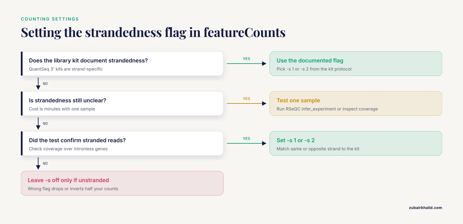
Subread's featureCounts assigns reads to features defined in a GTF annotation file, and it appears in both the Colab protocol [1] and PipeSeq [7]:
featureCounts -p -T 8 -t exon -g gene_id \
  -a GCF_000001405.40_GRCh38.gtf \
  -o counts/SRR21058845.counts.txt bam/SRR21058845.sorted.bam
Parameter notes:
-pdeclares paired-end input so fragments, not individual reads, are counted once.-t exon -g gene_idcounts reads overlapping exons and aggregates them by gene ID, which is the standard scheme for gene-level differential expression.- Add
-s 1(stranded, same strand) or-s 2(stranded, opposite strand) for stranded libraries, and leave it off only for unstranded libraries. This single flag is the most common silent error in the whole pipeline, and 3'-end stranded kits such as QuantSeq make it decisive [8].
Run this inside a loop over all BAM files, then merge per-sample count columns into one matrix. The final matrix has genes as rows, samples as columns, and raw integer counts as values. Keep the raw integers untouched. Normalization happens inside DESeq2.
Step 9: Differential expression with DESeq2
DESeq2 models raw counts with a negative binomial distribution and estimates fold changes across your groups. The neurodevelopmental rat study that compared maternal-separation animals to controls used DESeq with an adjusted P value cutoff below 0.05 and reported 202 differentially expressed genes, 128 upregulated and 74 downregulated, which is a realistic output scale for a two-group animal comparison [11].
library(DESeq2)

counts <- read.delim("counts/merged_counts.txt", row.names = 1, check.names = FALSE)
counts <- as.matrix(counts[, 7:ncol(counts)])   # skip featureCounts metadata columns

coldata <- data.frame(
  condition = factor(c("control", "control", "treated", "treated"),
                     levels = c("control", "treated"))
)
rownames(coldata) <- colnames(counts)

dds <- DESeqDataSetFromMatrix(countData = counts,
                              colData   = coldata,
                              design    = ~ condition)
dds <- dds[rowSums(counts(dds) >= 10) >= 2, ]   # keep genes with some signal
dds <- DESeq(dds)
res <- results(dds, contrast = c("condition", "treated", "control"))
res <- lfcShrink(dds, coef = "condition_treated_vs_control",
                 type = "apeglm", res = res)
write.csv(as.data.frame(res), "results_deseq2.csv")

sig <- subset(as.data.frame(res), padj < 0.05)
Reading the results table:
log2FoldChangeis the shrunken effect estimate. A value of 1.0 means a doubling of expression.padjis the false discovery rate adjusted P value. Filter onpadj, never on the raw P value, because thousands of simultaneous tests guarantee false positives otherwise.baseMeanis the normalized average expression. Genes with tinybaseMeanproduce unstable fold changes, which the low-count filter above removes.
The first rows of your results look like this (illustrative values):
              baseMean log2FoldChange  lfcSE    pvalue      padj
gene_symbol_A     1423          2.310 0.3121 2.1e-14 3.4e-11
gene_symbol_B       887         -1.872 0.2890 4.7e-12 5.1e-10
Quick visual checks catch most disasters before publication. Run a principal component plot of the variance-stabilized counts and confirm that replicate samples cluster by biological group, not by batch. Then plot a heatmap of the top varying genes and a volcano plot of the full result table, the same visualizations recommended in the minimal-hardware protocol [1]. If a control sample sits inside the treated cluster on the PCA plot, stop and investigate sample identities against the metadata before anything else.
For enrichment, submit the significant gene list to g:Profiler, the tool used for functional enrichment in the streamlined protocol [1], or use clusterProfiler in R. For non-model organisms with thin NCBI annotation, build a custom annotation package from NCBI genomic data and load it alongside clusterProfiler. This approach was demonstrated with a complete annotation package for Mycobacterium tuberculosis H37Rv, applied to differentially expressed genes from the rifampicin-response series GSE292409, and it avoids the annotation errors that blind homology transfers introduce [2].
When the Standard Pipeline Needs Adjusting
Non-model organisms without a reference genome
When no genome exists, assemble the transcriptome de novo, assess it, and annotate against NCBI's nr protein database. A published tick salivary gland study assembled roughly 25 million reads per replicate, clustered the assembly with CD-HIT at 95 percent identity and 90 percent coverage to about 50,231 non-redundant transcripts, scored 86 percent completeness with BUSCO, and then searched the proteins against NCBI nr before differential expression analysis [10]. The same principles extend to building custom R annotation packages for enrichment analysis in bacteria and other poorly annotated species [2].
Gene model confusion in well-annotated organisms
Even model-adjacent organisms suffer from competing gene sets. In the red flour beetle, the NCBI gene models and the community OGS3 models overlapped directly in only 50 to 57 percent of cases after a genome assembly update, which forced the BeetleAtlas resource to run both annotation tracks in parallel and let researchers compare expression patterns against read coverage in a genome browser to resolve disagreements [12]. The lesson generalizes: always record which GTF file version you used, and expect count tables to change when annotations change.
Bulk RNA-seq from heterogeneous tissue
Bulk RNA-seq measures an average across every cell in the sample, so a shift in cell composition can masquerade as a gene expression change. The myometrial labor study attributed part of its lower differentially expressed gene counts in early labor to bulk tissue heterogeneity rather than transcription alone [9]. Two remedies exist. Cell-type deconvolution estimates composition from bulk data using a single-cell reference, and one open-source workflow applied it to baboon kidney cortex bulk RNA-seq with 274 kidney cell-type marker transcripts, confirming that sex differences in expression were not explained by sampling differences [5]. Genomic deconvolution against curated signature sets works similarly in disease contexts, as shown in the ALS analysis that linked connexin-43 correlated genes to microglial activation signatures [13]. Both approaches are recommended as a rigor check for bulk studies of complex tissue [5].
Single-cell RNA-seq downloads
Single-cell datasets follow a different toolchain. The kidney stone scRNA-seq reanalysis pulled GSE176155 from GEO, processed raw FASTQ files through Cell Ranger v6.0.1 aligned to GRCh38, and completed quality control, normalization, PCA, UMAP, and graph-based clustering in Seurat v4.0.5 with differential expression by Wilcoxon rank-sum test and Bonferroni correction [4]. The hepatocellular carcinoma studies built on GSE158723 and GSE112271 followed the same GEO-to-Seurat pattern and validated the computational findings with immunofluorescence in patient tissue [14]. Budget for much larger disk space and memory than bulk analysis, because single-cell matrices hold tens of thousands of cells.
Machine learning on GEO matrices
Processed GEO matrices can feed predictive models when raw reads are secondary to the question. An autism spectrum disorder study downloaded 20 ASD and 19 typically developing samples from NCBI GEO, preprocessed them in R, and trained random forest and XGBoost classifiers, with the XGBoost model reaching about 67 percent five-fold cross-validated accuracy and surfacing the TCTA gene in both models' top signatures [15]. Read that accuracy number as a caution as much as a result, since modest cross-validated performance on small public cohorts is the norm, not a failure of method.
Key Parameters and Formulas at a Glance
| Step | Tool | Key setting | What it controls |
|---|---|---|---|
| Download | fasterq-dump | -e 6, -O dir | Parallel jobs and output location |
| Trim | Trimmomatic | SLIDINGWINDOW:4:15, MINLEN:36 | Quality window and minimum read length |
| Align | HISAT2 | -p, -x, -rna-strandness | Threads, index prefix, strand mode |
| Align QC | samtools flagstat | overall alignment rate | Sanity threshold above roughly 80 percent |
| Count | featureCounts | -p, -s 1 or -s 2, -g gene_id | Pairing, strandedness, gene aggregation |
| Statistics | DESeq2 | padj < 0.05, lfcShrink | False discovery control and effect size |
| Enrichment | g:Profiler, clusterProfiler | background gene universe | Which gene set the test compares against |
The background universe setting deserves emphasis. If you enrich only the genes that survived your count filter but pass the whole genome as background, every enrichment result skews toward highly expressed genes. Pass the filtered gene universe that entered the DESeq2 test.
Practical Tips for NCBI Gene Expression RNA-seq Work
- Write the pipeline as a shell script from day one. Every command in this guide chains cleanly into a single script, and PipeSeq's designers built their tool around exactly these standard steps partly because hand-run analyses are hard to reproduce across studies [7]. A script is your reproducibility record.
- Match the genome and GTF versions exactly. A mismatch between assembly versions produces featureCounts errors or zero-count genes. Record the NCBI assembly accession in your notes.
- Keep raw counts immutable. Save the featureCounts output untouched, and let DESeq2 or TPM conversion derive from copies. Published pipelines that normalize to TPM for visualization keep raw counts for the statistics, and the streamlined protocol handles both normalization to TPM and differential expression with pyDESeq2 in the same project [1].
- Verify strandness empirically when unsure. Align one sample and inspect read coverage across strongly expressed, intronless genes, or run a tool such as RSeQC's infer_experiment. The cost is minutes, and it prevents the strandedness error described above.
- Read the associated data descriptor before reanalysis. Descriptor papers disclose the kit, the sequencing platform, and the sampling scheme, such as the automated phenotyping and irrigation control behind the maize mycorrhiza dataset [8], which no amount of computational cleverness recovers from the FASTQ files.
- Work on cloud hardware for one-off projects. The Colab-based protocol removes the local hardware barrier entirely and is a reasonable default for a first full run [1].
Common Mistakes and Limitations
- Confusing accession types. Running
prefetch GSE292409fails, because prefetch expects SRR run accessions. A GSE series contains GSM samples, which contain SRR runs. Convert through the Run Selector before downloading. - Ignoring library strandedness. Unstranded counting on stranded libraries can drop or invert half your counts. The QuantSeq 3' kit used in the maize dataset is strand-specific, and any pipeline that ignores this measures the wrong strand [8].
- Using TPM or FPKM as DESeq2 input. DESeq2 requires raw integer counts and performs its own normalization. Feeding it pre-normalized values invalidates the dispersion model and the statistics.
- Trusting processed GEO matrices blindly. Processed values arrive in assorted normalizations, a compatibility problem that motivated PipeSeq's authors to standardize their own pipeline end to end [7]. When possible, start from raw reads so you control every step.
- Pooling GEO datasets without batch control. The PDAC meta-analysis succeeded because hub genes were concordant across seven datasets plus a new cohort, and the concordance itself was the evidence [6]. Naively merging count matrices from different labs, platforms, and library kits without a batch-aware design produces batch artifacts dressed up as biology.
- Overlooking cell composition in bulk tissue. A differential expression signal can reflect a different mix of cell types rather than regulation within cells, a limitation documented directly in myometrial bulk data [9] and addressable with deconvolution against single-cell references [5].
- Overfitting machine learning on small GEO cohorts. Cross-validated accuracy near two-thirds on a 39-sample cohort means the model is a hypothesis generator, not a diagnostic, and any candidate biomarkers need independent validation [15].
- Mixing gene model versions across analyses. As the Tribolium comparison showed, two authoritative gene sets for the same organism can agree on only about half of genes, so results are only as comparable as the annotations behind them [12].
- Skipping per-sample QC plots. A single failed library drags whole comparisons toward the null. PCA and alignment-rate tables belong in your records for every sample, not just the final report.
One limitation sits outside the pipeline entirely. Public datasets reflect the original authors' tissue collection, library preparation, and analysis goals, so a reanalysis can answer only questions the raw data can support, and individual research questions, particularly clinical ones, need domain expertise on top of computational work.
Frequently Asked Questions
Do I need raw FASTQ files, or can I use GEO's processed matrix?
For differential expression on a processed count matrix, the GEO matrix can suffice if it holds raw or normalized counts with sensible metadata. For quality control, alignment, novel transcript discovery, or anything downstream of reads, download the FASTQ files from SRA.
How much disk space and memory does this workflow need?
A typical bulk RNA-seq sample consumes several gigabytes of FASTQ plus tens of gigabytes of alignment files during processing, and DESeq2 runs comfortably in 16 GB of RAM for tens of samples. Delete intermediate SAM files immediately after sorting, and use a free Colab session if local hardware falls short [1].
Which aligner and counting tool combination should I use?
HISAT2 plus featureCounts is the combination used across published streamlined workflows [1][7], with STAR plus featureCounts and Salmon-based quantification as common alternatives. Consistency within a project matters more than the specific choice.
How do I handle an organism with no reference genome?
Assemble transcripts de novo, cluster redundant sequences, assess completeness with BUSCO, and annotate against NCBI nr, following the tick sialotranscriptome workflow [10], then build custom annotation packages for enrichment analysis in R [2].
Why does my featureCounts output have a strange first column full of semicolons?
The first columns of a featureCounts output hold gene identifiers and aChr-annotated metadata separated by tab characters, and multi-mapping assignments can join several gene IDs. Start your DESeq2 read at the correct numeric column and set check.names = FALSE in R, as shown in the code above.
Can I combine samples from two different GEO series in one analysis?
Only with a design that models batch or study as a covariate, and only when library kits, genome builds, and read types match. Concordance across datasets, as demonstrated in the PDAC hub-gene meta-analysis, is evidence in itself and a safer strategy than blind pooling [6].
What is the fastest way to sanity-check my differential expression results?
Three checks catch most errors. The PCA plot should cluster replicates by condition, housekeeping genes should sit near zero log2 fold change, and known positive controls from the literature for your treatment should appear in the significant list with the expected sign.
How do I cite or credit a dataset I downloaded from NCBI?
Cite the GEO series accession, the BioProject accession where present, and the associated publication listed on the series page. Data descriptor papers such as those accompanying the maize and zebrafish datasets exist specifically to be cited as the dataset's documentation [8][3].
Sources
- Streamline Protocol for Bulk-RNA Sequencing: From Data Extraction to Expression Analysis.
- Enhanced RNA-Seq Expression Profiling and Functional Enrichment in Non-model Organisms Using Custom Annotations.
- Transcriptomic data of larval zebrafish exposed to environmentally relevant levels of uranyl nitrate and sodium arsenite.
- Expression analysis of epithelial membrane protein 1 (EMP1) gene in kidney stone patients.
- Cell-type deconvolution of bulk RNA-Seq from kidney using opensource bioinformatic tools.
- Dysregulated expression of cell cycle regulators CDC20, PLK1, BUB1, CDC45, CDCA5 in pancreatic ductal adenocarcinoma.
- Development and validation of the PipeSeq program for RNA-seq data analysis in the Chlamydomonas reinhardtii as a model.
- Illumina RNA-seq data of Genotype-specific responses of maize plants to Funneliformis mosseae.
- Labour classified by cervical dilatation & fetal membrane rupture demonstrates differential impact on RNA-seq data for human myometrium tissues.
- De novo assembly of sialotranscriptome of Hyalomma anatolicum and insights into expression dynamics in response to Theileria annulata infection.
- Transcriptome profile analysis of genes by RNA-sequencing in neonatal maternal separation rats with autistic-like behaviors.
- BeetleAtlas 2: An enhanced Tribolium castaneum web resource for tissue and developmental transcriptomics allowing refinement of gene predictions.
- GJA1/CX43 High Expression Levels in the Cervical Spinal Cord of ALS Patients Correlate to Microglia-Mediated Neuroinflammatory Profile.
- scRNA-Seq Analysis Revealed CAFs Regulating HCC Cells via PTN Signaling.
- Identification of Potential Biomarkers in ASD Integrating RNA Seq Data and Machine Learning Approaches.