NCBI Gene Expression Data: Step-by-Step Guide
By Dr. Zubair Khalid, DVM, MS, PhD ·

By the end of this guide you will be able to find a gene expression study in NCBI's Gene Expression Omnibus (GEO), download its raw and processed files, load the data into R, run a differential expression analysis with GEO2R or limma, pull raw sequencing reads from the Sequence Read Archive (SRA), and validate the genes that come out of the analysis. You need a computer with an internet connection, R 4.0 or later with RStudio, and, for sequencing data, the SRA Toolkit. The command line examples use wget and curl, which ship with most systems. Everything named here is free.
This is a step-by-step guide, so each stage builds on the last. NCBI gene expression data live in GEO, an international public repository that archives gene expression and epigenomics data sets generated by microarray and next-generation sequencing technologies. GEO handles raw data files, processed data files, and descriptive metadata for more than 200,000 studies and 6.5 million samples, all of which are indexed, searchable, and downloadable [1].
What NCBI Gene Expression Data Is
GEO is built and maintained by the National Center for Biotechnology Information (NCBI), a division of the National Library of Medicine [1]. Researchers deposit data under widespread journal and funder mandates that require public sharing [1]. The repository was created in response to the demand for a public home for high-throughput gene expression data, and it is designed to act as a central distribution hub that complements in-house databases rather than replace them [2][3].
GEO is not one big table. It is a structured archive built around three central entities designed with expression and genomic hybridization experiments in mind [2]:
- Platform. A list of probes that defines which molecules an experiment can detect. A probe is a sequence-defined, anchored feature, such as an oligonucleotide spot on a microarray.
- Sample. A description of the molecules being probed, tied to exactly one platform, carrying the molecular abundance measurements.
- Series. The organization of samples into the meaningful data sets that make up one experiment.
Each entity carries a stable accession prefix, and the prefixes tell you what you are looking at before you click.
| Prefix | Entity | What it holds | Example |
|---|---|---|---|
| GSE | Series | One complete experiment with its samples, metadata, and files | GSE74000, an acetaminophen toxicity study [4] |
| GSM | Sample | One sample's abundance values and metadata | One row in a series samples table |
| GPL | Platform | Probe or feature definitions for an array or sequencing design | GPL570, the Affymetrix Human Genome U133 Plus 2.0 Array |
| GDS | DataSet | An NCBI-curated subset of a series with a defined comparison | GDS plus a number |
A microarray is a slide carrying thousands of fixed, sequence-defined probes that measure nucleic acid abundance in parallel. An RNA-seq experiment sequences the RNA itself. In GEO, microarray series store probe-level intensities, while RNA-seq series store processed matrices in GEO and raw reads in SRA. The two archives are used together at scale. ARCHS4, a resource that compiles all RNA-seq data deposited into SRA, shows how raw reads and GEO metadata combine into large reusable databases [5].
How to Use NCBI: Finding Your Way Around GEO
Open https://www.ncbi.nlm.nih.gov/geo/. The search box queries GEO DataSets through NCBI's Entrez system, the same unified search engine that runs PubMed and the Gene database. GEO sits alongside those databases in the broader NCBI collection, and series pages cross-link to the source publication, the organism taxonomy, and SRA run accessions.
Useful search patterns:
acetaminophen AND homo sapiens[organism]finds human studies mentioning acetaminophen.GSE74000[ACCN]jumps straight to one accession.- Left sidebar filters narrow results by organism, entry type (Samples, Series, DataSets, Platforms), and sample count.
Two related interfaces matter for expression work. GEO DataSets indexes experiment-level entries, including the curated GDS DataSets that NCBI staff assemble with defined sample groups and comparisons. GEO Profiles indexes gene-level expression charts, so you can search a gene symbol and see how that gene behaves across every sample of a series. The GEO DataSets and GEO Profiles interfaces exist specifically to make the microarray and sequencing archives mineable, and NCBI documents how to combine them for retrieval and analysis [6].
If you plan repeated or automated queries, skip the browser and use NCBI's E-utilities application programming interface, covered in Step 3.
Step 1: Find a Series That Fits Your Question
Start from the biology, not the accession. Write down the comparison you want, for example treated cells versus control cells, or diseased tissue versus healthy tissue. Then search GEO DataSets with the condition, the organism, and the entry type filter set to Series.
Check five things before you commit to a series:
- Organism and tissue match your question.
- Sample count supports the comparison. Three samples per group supports a simple two-group test. It does not support a machine learning model.
- Platform is one you can interpret. GPL570, the Affymetrix Human Genome U133 Plus 2.0 Array, is a common human microarray with 54,675 probe sets.
- Design in the Overall design field matches the comparison you wrote down.
- Raw data availability. Look for supplementary raw files or SRA links if you plan your own pipeline.
Published work shows the range of what a single series can support. GSE74000 contains transcriptomic profiles of liver samples from patients with acetaminophen-induced acute liver failure plus several hepatic cell systems exposed to acetaminophen, deposited with both raw and normalized microarray data [4]. GSE92563 is a time course in mouse colon after exposure to the food additive E171, with samples at 2, 7, 14, and 21 days [7]. GSE30531 holds longitudinal clinical trial microarray data that was later reused for predictive modeling [8]. Meta-analyses combine several series. As one example, four prostate cancer data sets, GSE55945, GSE104749, GSE46602, and GSE32571, were downloaded from GEO and analyzed together to identify differentially expressed genes [9].
Step 2: Read the Series Page Before You Download
Every series page follows the same layout. Read it in this order:
- Summary and Overall design. The submitters describe the experiment and the comparison in their own words.
- Samples table. Each row is one GSM sample with its title, source name, and Characteristics fields. The Characteristics fields are unstructured free text, which is the main reason sample metadata in GEO is hard to use at scale, a limitation addressed by curation projects such as STARGEO [10].
- Platform link. Opens the GPL page with the full probe table, including gene assignments.
- Data processing section. Describes exactly how the submitter produced the processed values. Read this to learn whether the matrix holds raw counts, normalized intensities, or log-transformed ratios.
- Supplementary file links. Raw archives, processed tables, and, for many RNA-seq studies, count matrices computed uniformly by NCBI [1].
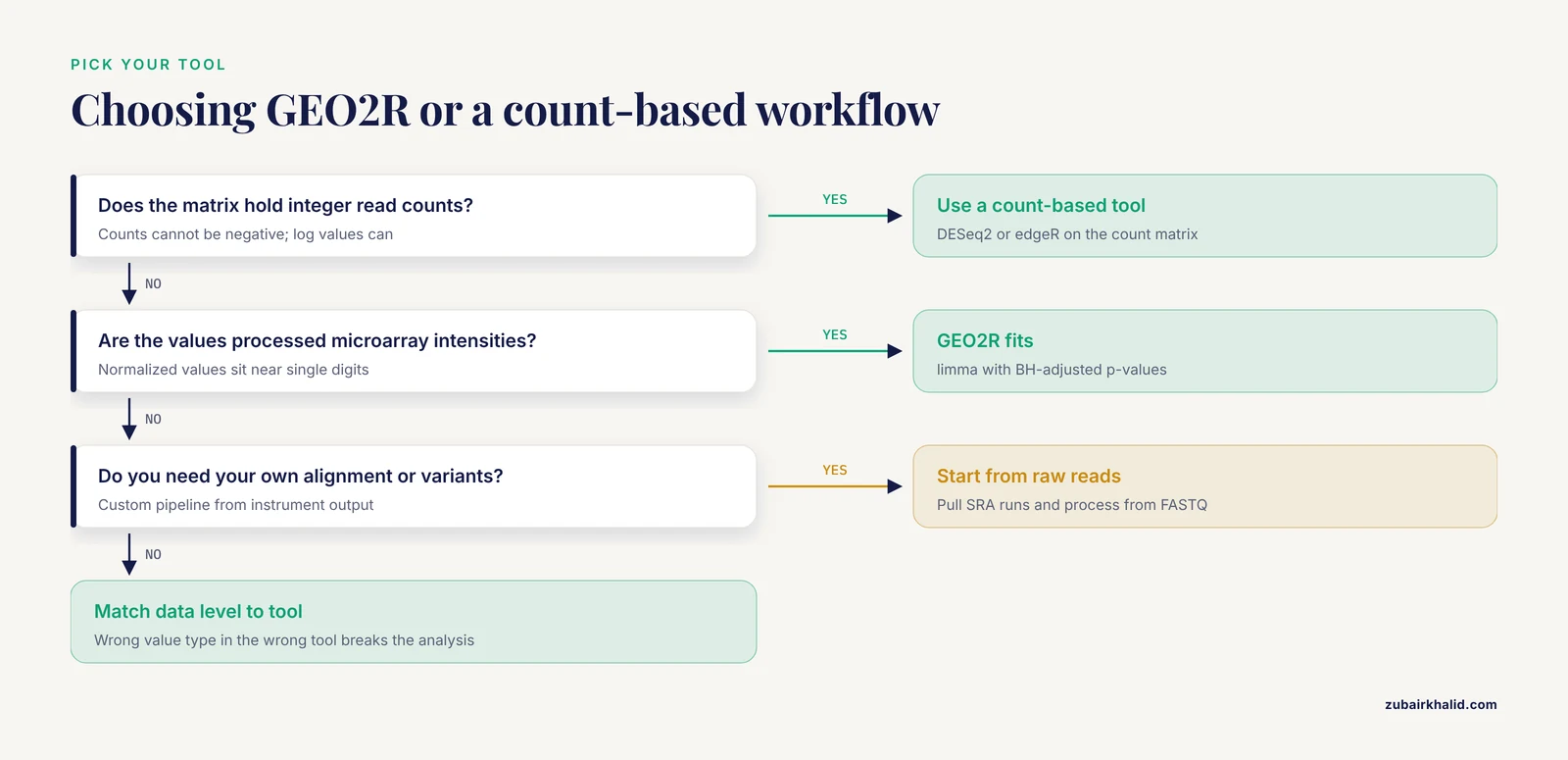
Metadata means the descriptive information attached to each sample, such as tissue, treatment, and donor. Decide at this point which data level you need, because it determines the tool. Quick differential expression on processed values needs only the series matrix. A full pipeline from raw instrument output needs the raw archive or SRA reads.
Step 3: Download the Files You Need
GEO stores several file types per series, and each answers a different need.
| File | What it holds | When to use it |
|---|---|---|
Series matrix (*_series_matrix.txt.gz) | Expression values plus all sample metadata in one compressed text file | Fast loading in R or Python |
| Processed supplementary tables | The submitter's per-sample expression tables | Reproducing the paper's numbers |
Raw archive (*_RAW.tar) | Instrument output such as CEL files, the raw intensity format for Affymetrix arrays | Your own normalization pipeline |
| NCBI count matrices | Uniformly computed gene counts for thousands of RNA-seq studies [1] | Count-based RNA-seq analysis without reprocessing |
| SRA runs | Raw sequencing reads in FASTQ format | Custom alignment, quantification, and variant work |
FASTQ is the standard text format for raw sequencing reads, with four lines per read, the sequence identifier, the sequence itself, a separator, and per-base quality scores.
Browser route. Scroll to the bottom of the series page and use the Download family links. For a quick look, this is enough.
Command line route. GEO organizes files by accession folder, built by replacing the last three digits of the accession with nnn. GSE74000 lives in the GSE74nnn folder.
wget https://ftp.ncbi.nlm.nih.gov/geo/series/GSE74nnn/GSE74000/suppl/GSE74000_series_matrix.txt.gzExpected output, with file sizes varying by series:
HTTP request sent, awaiting response... 200 OK
Saving to: 'GSE74000_series_matrix.txt.gz'

GSE74000_series_matrix.txt.gz  100%[==================>]   5.20M  9.1MB/s  in 0.6s

'GSE74000_series_matrix.txt.gz' saved
Inspect the metadata headers to confirm you grabbed the right study:
zcat GSE74000_series_matrix.txt.gz | head -n 40You will see lines in this format:
!Series_title	"Gene expression data from acetaminophen-induced toxicity in human hepatic in vitro systems and clinical liver samples"
!Sample_title	"..."
!Sample_characteristics_ch1	"..."
For raw microarray files, download and unpack the raw archive:
wget https://ftp.ncbi.nlm.nih.gov/geo/series/GSE74nnn/GSE74000/suppl/GSE74000_RAW.tar
tar -xf GSE74000_RAW.tar
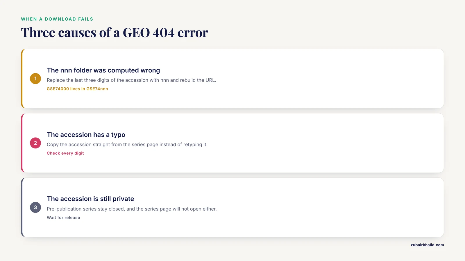
The 404 error. A mistyped URL returns this:
HTTP request sent, awaiting response... 404 Not Found
ERROR 404: Not Found.
Three causes cover almost every case. The nnn folder was computed wrong, so recompute it from the accession digits. The accession has a typo, so copy it from the series page. Or the accession is still private while the paper is in press, in which case the page itself will not open either.
Programmatic search. E-utilities lets scripts query GEO DataSets directly:
curl -s "https://eutils.ncbi.nlm.nih.gov/entrez/eutils/esearch.fcgi?db=gds&term=GSE74000[ACCN]&retmode=json"Expected output:
{
  "esearchresult": {
    "count": "1",
    "idlist": ["200074000"]
  }
}
NCBI assigns GSE entries unique identifiers (UIDs) in the 200000000 range, formed by adding 200000000 to the GSE number. Feed that UID to esummary.fcgi with db=gds to pull titles and metadata as JSON. For automated work, add the tool and email parameters so NCBI can contact you if your script misbehaves.
Step 4: Load the Data in R with GEOquery
GEOquery is the standard R package for pulling GEO series directly into R as ExpressionSet objects. An ExpressionSet is a Bioconductor structure that bundles expression values, sample metadata, and feature annotation in one object, which keeps the three pieces aligned.
install.packages("BiocManager")
BiocManager::install("GEOquery")

library(GEOquery)
gse <- getGEO("GSE74000", GSEMatrix = TRUE)
Parameters that matter:
GSEMatrix = TRUEreturns a list of ExpressionSet objects, one per platform, built from the series matrix files. This is the mode you want almost always. For a series measured on two platforms,gse[]andgse[]are the two matrices.getGPL = TRUE, the default, also downloads the platform table so probe IDs map to genes.destdirsets the cache folder. Point it at a project subfolder so repeated runs reuse the download.
Inspect what you loaded:
eset <- gse[[2]]
dim(exprs(eset))
head(pData(eset)$title)
head(featureNames(eset))
Expected output for the dimension call, where the sample count here is illustrative and must match the series page:
Features  Samples
   54675        24
The first number is the probe count, 54,675 for any GPL570 human array. The second number is the sample count. pData(eset) returns the sample metadata table, and featureNames(eset) returns the probe identifiers.
Run two quick quality checks before any statistics:
summary(exprs(eset)[, 1])
boxplot(exprs(eset), outline = FALSE, las = 2)
Raw microarray intensities sit in the hundreds to thousands. Normalized values sit near single digits and look similar across samples. If one sample's box sits far from the rest, flag that sample now, because it will distort everything downstream.
Three errors you will hit:
Error in library(GEOquery) : there is no package called 'GEOquery'. The package is not installed. Run the BiocManager line above and reopen the library.- GEOquery stops with
cannot open URLfollowed by the address it tried. This is a network, proxy, or transient server issue. Retry, or download the series matrix manually with wget and load the local file. Error: cannot allocate vector of size 1.8 Gb. R ran out of memory. Load one platform at a time, read the compressed matrix with data.table's fread, or move to a machine with more RAM.
Verify the result before moving on. The dimensions match the series page, the pData columns include the Characteristics fields you saw on the page, and the expression values fall in a plausible range for the platform.
Step 5: Analyze Differential Expression with GEO2R
GEO2R is the analysis tool built into compatible series pages. It applies limma, an R package that fits a linear model per gene and moderates variance estimates across genes, then reports log2 fold changes and Benjamini-Hochberg adjusted p-values. The adjusted p-value controls the false discovery rate, the expected proportion of false positives among the genes you call significant. The 2023 GEO update added interactive graphical plots in GEO2R that help users identify differentially expressed genes and assess data set quality in the browser [1].
Walkthrough on a series page:
- Click Analyze with GEO2R under the series.
- In the samples table, select the control samples, assign them to Group A, and rename the group. Then select the treated samples and assign Group B. GEO2R needs at least two samples per group to estimate variance.
- Open Options. The adjustment method defaults to BH, short for Benjamini-Hochberg. Keep the default unless you have a specific reason to change it.
- Click Top Differential Expression. The table lists the top 250 genes by default with columns ID, adj.P.Val, P.Value, t, B, logFC, and gene symbol when the platform supports mapping. Here t is the moderated t statistic and B is the log odds that the gene is truly differentially expressed.
- Open the interactive plots to check separation between groups and spread within groups.
- Click Save R script. This is the most valuable button in GEO2R, because it hands you the exact limma commands that reproduce the result on your own machine.
The equivalent analysis in R, once the series is loaded with GEOquery:
library(limma)
group <- factor(c("control", "control", "acetaminophen", "acetaminophen"))
design <- model.matrix(~ group)
fit <- lmFit(eset, design)
fit <- eBayes(fit)
top <- topTable(fit, number = 20, adjust.method = "BH")
head(top)
Parameters that matter:
designencodes the comparison. The formula~ groupcompares the second level against the first, ordered alphabetically by default, so name your levels deliberately.adjust.method = "BH"controls false discovery. With roughly 20,000 genes tested, unadjusted p < 0.05 expects about 1,000 false positives, which is why adj.P.Val is the column to filter.numbersets how many rows topTable returns.
Read the results like this. logFC is the log2 fold change, so logFC of 1 means expression doubled and -1 means it halved. Filter on adj.P.Val below 0.05 first, then rank by the size of logFC.
GEO2R works on processed microarray-style matrices and, by default, applies no background correction and no normalization, meaning it analyzes the processed values exactly as deposited. Some series, such as RNA-seq feature count tables, are not GEO2R compatible, in which case the tool is unavailable or warns you, and you should use a count-based workflow instead.
Step 6: Work With RNA-Seq Data and SRA Reads
RNA-seq series in GEO give you three options, in order of effort.
Option 1, NCBI's uniformly computed count matrices. GEO now generates consistently computed gene expression count matrices for thousands of RNA-seq studies [1]. They appear as supplementary files on the series page, named for the organism and genome assembly. A count matrix is a gene-by-sample table of integer read counts per gene. Because NCBI computes these with one standard pipeline, they remove a major source of between-study processing noise.
counts <- read.delim("the_exact_file_from_the_series_page.txt", row.names = 1)
dim(counts)
Then analyze with a count-based tool such as DESeq2:
library(DESeq2)
dds <- DESeqDataSetFromMatrix(countData = counts, colData = metadata, design = ~ condition)
dds <- DESeq(dds)
res <- results(dds)
head(res[order(res$padj), ])
The results table carries baseMean, log2FoldChange, lfcSE, stat, pvalue, and padj. Filter on padj, the adjusted p-value, exactly as you would in limma.
Option 2, submitter-processed matrices. Useful for reproducing a specific paper, but processing steps vary by lab, so read the Data processing section first.
Option 3, raw reads from SRA. Needed for custom pipelines, new alignments, or variant-level work. Install the SRA Toolkit, then:
prefetch SRR000001
fasterq-dump SRR000001
fastqc SRR000001_1.fastq SRR000001_2.fastq
prefetch downloads the run into a local cache, fasterq-dump writes FASTQ files, one per mate for paired-end data, and fastqc produces an HTML quality report per file. In the report, check per-base quality scores, adapter contamination, and overrepresented sequences before anything else.
One published end-to-end example shows the shape of a full pipeline. A study of allele-specific expression between Bos taurus and Bos indicus cows pulled RNA-seq reads from SRA, processed them with FASTQC and Trimmomatic, aligned them to the bovine reference genome with TopHat2, and called variants with Samtools [12]. Modern pipelines swap in newer aligners and quantifiers, but the order of operations is the same, quality control, trimming, alignment or pseudoalignment, then counting.
If fasterq-dump fails, it reports that it cannot locate the object. Check the SRR accession on the SRA page, confirm the run belongs to the study you think it does, and confirm the run is public.
Step 7: Pull Many Data Sets for Meta-Analysis
Single-series conclusions are fragile. Combining series is where public expression data pays off, and several tools exist for exactly that.
- COnTORT retrieves all available gene expression data and associated metadata for an organism from GEO and compiles them into text files ready for downstream bioinformatic applications [11]. Use it when you want everything for one organism in a single pass.
- ExAtlas is an online tool for meta-analysis and visualization that handles both your own data and data pulled from GEO. It runs fixed effects, random effects, z-score, and Fisher's method meta-analyses, plus gene set enrichment, gene set overlap, ANOVA, and PCA, with graphical outputs [13]. Use it when you want cross-study statistics without writing code.
- ARCHS4 compiles all RNA-seq data deposited into SRA into a searchable resource, supporting unbiased queries across thousands of samples [5]. A macrophage study used it to assemble an unbiased RNA-seq database and showed that commonly used polarization protocols produce distinct, non-interchangeable gene expression profiles [5].
- STARGEO tackles the free-text metadata problem with crowd-curated sample annotations across studies, which sharpens the groupings used in meta-analysis [10].
A concrete published example shows the payoff. Researchers downloaded four prostate cancer series from GEO, GSE55945, GSE104749, GSE46602, and GSE32571, identified 633 upregulated and 1,219 downregulated genes, 1,852 differentially expressed genes in total, and narrowed the list to key genes including EGFR, MYC, VEGFA, and PTEN [9]. Metadata-scale analysis works the same way outside human disease. Studies of the fungi Phanerochaete chrysosporium and Postia placenta retrieved many GEO data sets per organism and found consistent expression patterns of carbohydrate-active enzymes that only became visible when studies were combined [14][15].
When you combine series yourself, harmonize gene identifiers across platforms, map every probe to a gene with one stated rule, and model between-study variance rather than stacking matrices into one table.
Step 8: Validate Your Hits
Computational hits are hypotheses. Two validation routes are standard.
Experimental validation. If you follow up with RT-qPCR, verify primer specificity first. A bioinformatics workflow using NCBI Primer BLAST, in silico PCR in the UCSC genome browser, and the Ensembl DNA database evaluated 504 primer sets from 70 recent rat toxicological studies and found potential mismatches in 9 percent, cross-matches in 13.5 percent, co-amplification of multiple splice variants in 9 percent, and sub-optimal amplicon sizes in 25 percent [16]. The same study showed that lowly expressed genes are the most susceptible to genomic DNA contamination, so include no-reverse-transcriptase controls for weak signals [16]. Run the same checks before you order primers for genes pulled from GEO.
Computational validation. Re-test your gene list in an independent series you did not use for discovery. Machine learning studies built on GEO data show what independent testing looks like at scale. A Random Forest classifier trained on 15 autism spectrum disorder and 15 typical development samples from GEO reached 96.67 percent accuracy, sensitivity, and specificity in 5-fold cross-validation [17]. A sepsis study merged microarray series from GEO and ArrayExpress into one meta-expression set and compared differential expression against decision tree, random forest, support vector machine, and deep learning classifiers, with the best models exceeding 0.96 accuracy and 0.99 area under the curve [18]. A diabetes study profiled gene expression with support vector machine, random forest, K-nearest neighbors, and logistic regression, combining random forest with logistic regression for its final model [19]. For marker discovery specifically, the Bioconductor package MGFM predicts tissue and cell type marker genes from microarray data and was validated against GEO tissue series covering brain, heart, kidney, liver, and lung [20].
Practical Tips for NCBI Gene Expression Data
- Record provenance in your script. Put the GSE accession, file names, and download date in a comment header. Submitters can update files, so future-you needs to know which version you analyzed.
- Set
destdirin GEOquery to a project folder so re-runs reuse the cache instead of re-downloading. - Read the Data processing block before choosing a tool. It tells you whether the matrix is raw, normalized, or log-transformed, which decides between limma, DESeq2, or edgeR.
- Use the saved GEO2R script as your starting pipeline, then extend it rather than rebuilding from scratch.
- Add
toolandemailparameters to automated E-utilities calls so NCBI can reach you if a script misbehaves. - Match the data level to the question. Processed matrices answer differential expression questions fast. Raw reads answer alignment, variant, and novel transcript questions.
- Keep downloaded files read-only and work on copies, so a bad overwrite never costs you a re-download.
- Search GEO Profiles by gene symbol when you want to see one gene's behavior across a whole series before committing to a full analysis.
Common Mistakes and Limitations
- Treating the series matrix as raw data. For most microarray series, the series matrix holds submitter-processed values, and raw intensities live in the raw archive. Running a raw-data pipeline on processed values double-normalizes the data.
- Feeding the wrong value type into the wrong tool. Integer counts belong in count-based tools such as DESeq2 or edgeR. Continuous normalized intensities belong in limma-style tools. Log-transformed values can be negative and counts cannot, which is the fastest visual check of what you are holding.
- Trusting column order or free-text labels. Verify sample groups against the Characteristics fields, which are unstructured free text [10]. Two studies of the same disease can use incompatible labels for the same phenotype, and even within one system, protocol labels are not interchangeable [5].
- Ignoring the platform. Probe IDs are meaningless without the GPL annotation table, and one probe can map to several genes. Map probes to genes explicitly and report the mapping rule.
- Skipping multiple testing correction. A genome-wide analysis runs tens of thousands of hypotheses at once. Filter on adjusted p-values, never on raw p-values alone.
- Pooling studies without accounting for batch and platform. Platforms define different probe sets, and labs differ in processing. Use meta-analysis methods that model between-study variance [13] instead of stacking matrices into one table.
- Assuming GEO2R fits every data type. GEO2R targets processed microarray-style matrices. RNA-seq counts need count-based models.
- Downloading raw reads when processed data would answer the question, or the reverse. Reprocessing is expensive, and for very large series, submitter-processed values are sometimes the only practical route.
- Overinterpreting small series. A 15-versus-15 comparison can support a classifier but not a definitive biomarker panel. Report uncertainty and validate externally.
- Forgetting that GEO stores what submitters deposit. Annotation quality varies, and metadata errors propagate into reanalyses. Curated and crowd-curation resources exist precisely because of this [10].
Limitations. Every result in this workflow is computational. Differentially expressed genes from GEO reanalysis are candidate findings that need experimental confirmation, and RT-qPCR follow-up only counts as confirmation when primer specificity and RNA quality controls are verified first [16]. Individual biological conclusions require domain expertise and laboratory validation.
Frequently Asked Questions
What is the difference between GEO and SRA?
GEO stores processed expression matrices, sample metadata, and platform definitions, while SRA stores the raw sequencing reads. Most RNA-seq series in GEO link to SRA run accessions, so you can move from summary data down to raw FASTQ files when you need them.
What do the prefixes GSE, GSM, and GPL mean?
GSE is a series, the complete experiment. GSM is a single sample within that series. GPL is the platform, the list of probes or features used to measure the samples. One GSE contains many GSMs, all tied to one or more GPLs.
Can I download NCBI gene expression data without writing code?
Yes. Every series page has browser download links for the series matrix and supplementary files, and GEO2R runs a complete differential expression analysis in the browser with no local software installed.
How do I cite a GEO series?
Include the GSE accession in your methods section and cite the original publication linked on the series page. The accession lets any reader retrieve the exact data you used.
Why does a series have both raw and processed files?
Submitters deposit raw instrument output plus their own processed values. Raw files let you apply your own pipeline, and processed files let you reproduce or extend the paper's analysis quickly.
Can GEO2R analyze RNA-seq data?
GEO2R is designed for processed microarray-style matrices. For RNA-seq, download GEO's uniformly computed count matrices or the raw reads, then use a count-based workflow such as DESeq2 or edgeR.
How do I find every expression data set for one organism?
Search GEO DataSets with the organism filter, or use a bulk retrieval tool such as COnTORT, which pulls all available expression data and metadata for an organism from GEO into text files.
What should I do if a GEO download returns a 404 error?
Check the accession folder in the URL, which replaces the last three digits of the GSE number with nnn. A wrong folder, a typo in the accession, or a private pre-publication accession all produce the 404. Verify the accession on the series page first.
Sources
- NCBI GEO: archive for gene expression and epigenomics data sets: 23-year update.
- NCBI gene expression and hybridization array data repository
- Gene Expression Omnibus: NCBI gene expression and hybridization array data repository
- Gene expression data from acetaminophen-induced toxicity in human hepatic in vitro systems and clinical liver samples
- Leveraging a comprehensive unbiased RNAseq database to characterize human monocyte-derived macrophage gene expression profiles within commonly employed in vitro polarization methods
- Mining microarray data at NCBI's Gene Expression Omnibus (GEO)*.
- Time course gene expression data in colon of mice after exposure to food-grade E171
- Bayesian state-space modeling in gene expression data analysis: An application with biomarker prediction.
- Identification of Potential Key Genes in Prostate Cancer with Gene Expression, Pivotal Pathways and Regulatory Networks Analysis Using Integrated Bioinformatics Methods
- Precision annotation of digital samples in NCBI’s gene expression omnibus
- COnTORT: COmprehensive Transcriptomic ORganizational Tool for Simultaneously Retrieving and Organizing Numerous Gene Expression Data Sets from the NCBI Gene Expression Omnibus Database
- Allele Specific Expression (ASE) analysis between Bos Taurus and Bos Indicus cows using RNA-Seq data at SNP level and gene level.
- EXATLAS: AN INTERACTIVE ONLINE TOOL FOR META-ANALYSIS OF GENE EXPRESSION DATA
- Metadata Analysis of Phanerochaete chrysosporium Gene Expression Data Identified Common CAZymes Encoding Gene Expression Profiles Involved in Cellulose and Hemicellulose Degradation
- Molecular Networks of Postia placenta Involved in Degradation of Lignocellulosic Biomass Revealed from Metadata Analysis of Open Access Gene Expression Data
- A bioinformatics workflow for the evaluation of RT-qPCR primer specificity: Application for the assessment of gene expression data reliability in toxicological studies.
- Differential Gene Expression Data Analysis of ASD Using Random Forest
- Comparison of machine-learning methodologies for accurate diagnosis of sepsis using microarray gene expression data
- Diabetes Insights: Gene Expression Profiling with Machine Learning and NCBI Datasets
- MGFM: a novel tool for detection of tissue and cell specific marker genes from microarray gene expression data