NCBI Datasets Command-Line Tool
By Dr. Zubair Khalid, DVM, MS, PhD ·

By the end of this NCBI Datasets command line tutorial you will be able to install the datasets and dataformat utilities, download reference genomes for any taxon, flatten metadata into spreadsheet-ready tables, pull gene sequences and ortholog sets, query the NCBI Taxonomy database from the shell, and wrap all of it into a reproducible script. Everything runs locally from your terminal, which means no click-by-click browsing and no copy-pasting accessions by hand.
You need a Unix-like shell (Linux, macOS, or Windows Subsystem for Linux), Conda or Miniconda installed, roughly 200 MB of free disk space for the examples here, and an internet connection. A text editor and basic familiarity with grep and awk help but are not required.
What the NCBI Datasets Command-Line Tool Is
NCBI Datasets is the National Center for Biotechnology Information's unified access layer for biological sequences, annotations, and metadata across taxa. It was designed around FAIR principles (findable, accessible, interoperable, reusable) and delivers data as coherent packages of sequences plus metadata rather than as loose individual files [1]. Two programs make up the command-line side of this resource:
datasetsqueries NCBI and downloads data packages as zip archivesdataformatconverts the JSON reports inside those packages into CSV, TSV, or XLSX tables
The tool covers several data domains. The genome domain retrieves assemblies and their annotation files. The gene domain retrieves gene records, coding sequences, proteins, and ortholog relationships computed across eukaryotic genomes by the NCBI Orthologs pipeline [2]. The taxonomy domain retrieves organism names, classifications, ranks, and identifier cross-references, a capability that expanded substantially in 2024 when NCBI extended programmatic access to taxonomic information through the command-line tools and APIs [3]. A virus genome domain supports SARS-CoV-2 and related viral data.
If you are building a broader guide to how to use NCBI resources programmatically, the Datasets tools sit alongside older interfaces such as Entrez Direct and alongside specialized tools for other databases. For example, pysradb provides command-line access to Sequence Read Archive metadata and raw read data [4], and TaxonKit offers fast TaxId and lineage manipulation built on the same NCBI Taxonomy dump files [5]. Knowing which tool owns which database is the first step in a sane NCBI databases guide strategy. Datasets handles assemblies, genes, taxonomy summaries, and orthologs. It does not fetch raw reads.
Installing the Tools
Step 1: Install with Conda
The simplest route on Linux, macOS, and Windows Subsystem for Linux is Conda:
conda install -c conda-forge ncbi-datasets-cliThis installs both datasets and dataformat into the active environment. Verify the installation:
datasets --version
dataformat --version
Expected output looks something like this (your version numbers will differ):
v16.0.0
v16.0.0
Step 2: Alternative, Direct Binary Download
If you cannot use Conda, NCBI publishes prebuilt binaries on its public FTP site at the datasets command-line directory:
# Browse https://ftp.ncbi.nlm.nih.gov/pub/datasets/command-line/ for the current builds
curl -O https://ftp.ncbi.nlm.nih.gov/pub/datasets/command-line/v2/linux-amd64/datasets-linux-amd64.zip
unzip datasets-linux-amd64.zip
./datasets --version
Download the matching build for your platform (linux-amd64, macos-arm64, windows-amd64, and variants are published). Copy the executables to a directory on your PATH such as ~/.local/bin.
Step 3: Set an API Key
For anything larger than a handful of records, request an NCBI API key through your NCBI account settings and export it:
export NCBI_API_KEY=your_key_hereThe tool picks the variable up automatically and applies higher request limits. Add the export line to your ~/.bashrc or ~/.zshrc so it persists across sessions.
NCBI Datasets Command Line Tutorial: Step by Step
This walkthrough uses real commands with real expected outputs. Work through it in order. Each step builds on the previous one.
Step 1: Preview What a Taxon Contains Before Downloading
Always preview first. The summary subcommand returns a small JSON report with no download cost:
datasets summary genome taxon "Escherichia coli" --referenceThe output is JSON with a count field and a compact record list:
{
  "total_count": "1",
  "reports": [
    {
      "accession": "GCF_000005845.2",
      ...
That accession, GCF_000005845.2, is the well-known complete reference genome of E. coli K-12 substrain MG1655. The GCF prefix identifies a RefSeq assembly. A GCA prefix would identify a GenBank assembly, which is the unfiltered submission archive. Filtering to RefSeq and to reference status is the single most useful default behavior in genome work.
To see how many assemblies exist in total, drop the reference filter:
datasets summary genome taxon "Escherichia coli" --assembly-level completeStep 2: Download a Reference Genome Package
Download the full data package for that reference assembly:
datasets download genome taxon "Escherichia coli" \
  --reference \
  --include genome,protein,gff3,gbff,report \
  --filename ecoli-ref.zip
What each piece does:
download genome taxonselects assemblies by taxonomy name. You can substitute a TaxId such as562for the species name.-referencerestricts to reference assemblies only.-includeselects which file types land in the package. Valid values includegenome(the FASTA of the genomic sequences),protein(translated CDS products),gff3,gbff,rna, andreport.-filenamenames the output zip.
Expected console output:
Downloading: ncbi_dataset.zip... doneIf you omit -include, the tool downloads a sensible default set of files. If you want metadata only with no sequences, use -include none.
Step 3: Unpack and Inspect the Data Package
unzip ecoli-ref.zip -d ecoli-ref
find ecoli-ref -type f | head -20
The package always follows the same layout:
ecoli-ref/ncbi_dataset/data/dataset_catalog.json
ecoli-ref/ncbi_dataset/data/assembly_data_report.jsonl
ecoli-ref/ncbi_dataset/data/GCF_000005845.2/GCF_000005845.2_ASM584v2_genomic.fna
ecoli-ref/ncbi_dataset/data/GCF_000005845.2/..._protein.faa
ecoli-ref/ncbi_dataset/data/GCF_000005845.2/..._genomic.gff
ecoli-ref/ncbi_dataset/data/GCF_000005845.2/..._genomic.gbff
Two files matter for validation. dataset_catalog.json is the manifest. It lists every file the package was supposed to contain, which lets you verify completeness programmatically. assembly_data_report.jsonl is one JSON object per assembly with structured metadata, and it is the input that dataformat consumes in the next step.
A quick sanity check on the sequence file:
grep -c ">" ecoli-ref/ncbi_dataset/data/GCF_000005845.2/*_genomic.fnaThis prints the number of contigs or chromosomes in the assembly. For a complete bacterial genome you expect a small count, typically one chromosome plus a few plasmids.
Step 4: Flatten Metadata to a Table with dataformat
The JSONL report is machine friendly but not spreadsheet friendly. dataformat fixes that:
dataformat tsv genome \
  --inputfile ecoli-ref/ncbi_dataset/data/assembly_data_report.jsonl \
  --fields accession,organism-name,assembly-level,assembly-stats-total-sequence-length,assembly-stats-contig-n50 \
  --output-file assemblies.tsv
column -t -s $'\t' assemblies.tsvExpected output:
Accession      Organism name    Assembly level  Assembly stats total sequence length  Assembly stats contig N50
GCF_000005845.2  Escherichia coli  Complete Genome  4641652                             4641652
Run dataformat tsv genome, help to print the complete field vocabulary. Do not guess field names from memory. The same pattern applies to the other domains: dataformat tsv gene for gene packages, dataformat tsv taxonomy for taxonomy packages, and dataformat xlsx variants when a collaborator insists on Excel.
Step 5: Bulk Download by Taxon with Filters
The real power shows up when you need many genomes. This command grabs all complete RefSeq assemblies of the genus Listeria released since a given date:
datasets download genome taxon "Listeria" \
  --assembly-level complete \
  --released-since 2020-01-01 \
  --include genome,report \
  --filename listeria.zip
Useful filter options for the genome domain:
| Option | Effect | Typical use |
|---|---|---|
-reference | Keep only reference assemblies | One clean assembly per taxon |
-assembly-level | Filter to complete genome, chromosome, scaffold, or contig | Consistent comparability |
-released-since | Restrict to assemblies released after a date | Incremental updates |
-include | Choose package contents | Skip files you will not use |
-exclude-atypical | Drop assemblies flagged as atypical by NCBI quality rules | Screening out problematic assemblies |
-taxon | Restrict when the positional argument is an accession list | Mixed-identifier queries |
-dry-run | Preview the selection and file sizes before committing | Planning disk usage |
A word of caution about scale. If the summary count for your query is in the thousands, check -dry-run first and confirm you have disk space. Some bacterial genera now hold tens of thousands of assemblies.
Step 6: Work with Gene Records
Genes are fetched by GeneID, by symbol within a taxon, or by taxon-wide sweeps. BRCA1 has GeneID 672:
datasets summary gene gene-id 672Download the gene's coding sequence, protein, and transcript records plus the gene data report:
datasets download gene gene-id 672 \
  --include protein,cds,rna \
  --filename brca1.zip
To pull every protein-coding gene for an organism, use the taxon selector:
datasets download gene taxon "Drosophila melanogaster" \
  --include protein \
  --filename dmel-genes.zip
Because NCBI Orthologs assigns ortholog relationships gene by gene and integrates them into the NCBI Gene resource, the Datasets tools expose orthology directly [2]. Fetch the ortholog set for a gene like this:
datasets download gene ortholog 672 \
  --include protein \
  --filename brca1-orthologs.zip
The package contains a gene_data_report.jsonl describing each ortholog, including the species, symbol, and ortholog category, alongside the protein FASTA files. Convert the report to a table:
dataformat tsv gene \
  --inputfile brca1-orthologs/ncbi_dataset/data/gene_data_report.jsonl \
  --fields gene-id,symbol,tax-id,tax-common-name,ortholog-category \
  --output-file brca1-orthologs.tsv
Step 7: Query Taxonomy
The taxonomy domain returns names, ranks, lineages, and identifiers. The NCBI Taxonomy resource is the curated hub for organism names and classification, and Datasets now exposes it more fully across its web pages, command-line tools, and APIs [3].
Preview a node:
datasets summary taxonomy taxon "Apis mellifera"Download a subtree with its classification structure, useful for building custom lineage tables:
datasets download taxonomy taxon "Bombus" \
  --report tree,ids,name \
  --filename bombus-tax.zip
Convert the report and reformat lineages for downstream work:
dataformat tsv taxonomy \
  --inputfile bombus-tax/ncbi_dataset/data/taxon_data_report.jsonl \
  --fields tax-id,tax-common-name,formal-name,rank,genetic-code \
  --output-file bombus.tsv
If you need heavier lineage manipulation, such as lowest common ancestor computation or large-scale TaxId filtering, TaxonKit complements the Datasets tools well because it operates directly on the NCBI Taxonomy dump with seven dedicated subcommands [5]. If your downstream pipeline is a metagenomic classifier or an LCA profiler such as ngsLCA, which expects NCBI taxonomy inputs, exporting lineages from Datasets or TaxonKit feeds that step cleanly.
Step 8: Chain Commands into a Reproducible Script
A short shell script makes the whole retrieval reproducible:
#!/bin/bash
set -euo pipefail

TAXON="Escherichia coli"
OUT="ecoli_$(date +%Y-%m-%d)"

datasets download genome taxon "$TAXON" \
  --reference --include genome,gbff,report \
  --filename "$OUT.zip"
unzip -q "$OUT.zip" -d "$OUT"

dataformat tsv genome \
  --inputfile "$OUT/ncbi_dataset/data/assembly_data_report.jsonl" \
  --fields accession,organism-name,assembly-level,assembly-source,assembly-stats-total-sequence-length \
  --output-file "$OUT/assemblies.tsv"

grep -c ">" "$OUT"/ncbi_dataset/data/GCF_*/*_genomic.fna
Record three things alongside your analysis: the tool version from datasets, version, the date of the download, and the resulting dataset_catalog.json. Reference databases at NCBI grow continuously, and sequence database versioning is a recognized challenge for reproducibility because pipelines rerun months later will encounter different reference sets [6]. The catalog file plus the version stamp is your provenance record.
Step 9: Handling NCBI Annotation Formats Downstream
The annotation files in a genome package are standard GenBank formats. The gbff file opens in any GenBank-aware tool. The flat feature tables inside some NCBI submission pipelines, the .tbl files, occasionally need conversion for downstream schema such as UCSC track formats, and parsers exist for exactly that purpose [7]. For most work the GFF3 and protein FASTA files are what you actually feed into aligners, genome browsers, and annotation viewers.
Common Mistakes and Limitations
These are the errors that account for most failed first attempts, listed with their exact symptoms.
Wrong file type requested with, include. Symptom: Error: invalid value "fasta" for "-include". The value is genome, not fasta. Valid include values are genome, protein, rna, cds, gff3, gbff, report, seq-report, and none for the genome domain, with domain-specific sets elsewhere. Run the subcommand help to see the accepted list.
Unquoted taxon names. Symptom: Error: unable to parse taxon. datasets download genome taxon Escherichia coli passes Escherichia as the taxon and then coli as an unexpected positional argument. Always write "Escherichia coli".
Assuming the zip layout is stable across versions. The package structure has been stable for years but the manifest, not your memory, is the contract. Read dataset_catalog.json in scripts rather than hardcoding paths. If a package appears empty, the first thing to check is whether the catalog lists the files and whether the download completed. A partially downloaded zip fails to unzip with an error such as End-of-central-directory signature not found, and the fix is to delete the file and download again.
Guessing TSV field names. Symptom: dataformat exits with a message about an unknown field. Field names are versioned and hierarchical. Run dataformat tsv genome, help and copy names exactly.
Confusing reference with RefSeq. The -reference flag returns only the single designated reference assembly per species. To get all RefSeq assemblies, use -assembly-source refseq. To get all GenBank assemblies, use -assembly-source genbank.
Expecting raw reads. Datasets delivers assemblies, annotation, and metadata. Raw sequencing reads live in the Sequence Read Archive and require a different toolchain such as pysradb or the SRA Toolkit [4]. This is the most common expectation gap for users who arrive asking how to use NCBI for one-stop data retrieval.
Expecting bulk browser-style sequence pulls. Older workflows for tens of thousands of individual sequences relied on dedicated GUI tools such as the NCBI Mass Sequence Downloader [8]. Datasets replaces much of that need at the genome and gene level, but if your task is thousands of individual GenBank records by accession, Entrez Direct or Efetch remains the better fit.
Ignoring database drift. An assembly you downloaded last year may be replaced or suppressed. NCBI marks new assemblies with new accession versions, and pipelines that assume static references can silently shift behavior. This is the classic reason researchers archive and version reference databases locally [6]. Snapshot your packages and note versions.
Annotation format surprises. RefSeq .tbl feature tables are not directly consumable by every downstream tool. Known converters, for example the Tbl2KnownGene parser that produces UCSC knownGene format tables, exist for those specific needs [7]. Check what format your downstream tool requires before assuming any package file will drop in.
Forgetting the API key on large jobs. Symptoms include slow throughput on taxon-wide downloads. Export NCBI_API_KEY before large batches.
NCBI Datasets Command Line Tutorial Tips
A few habits that pay off in daily use.
Summarize before you download, every time. The summary subcommands cost seconds and tell you the record count before you commit to a download. Combine them with filters to shrink the selection in the preview, then carry those exact filters into the download command.
Prefer the report files over scraping FASTA headers. The *_data_report.jsonl files contain structured, normalized metadata. Parsing FASTA deflines for organism names is fragile because the header text varies between submission pipelines.
Use xlsx output for collaborators. dataformat xlsx genome produces a formatted spreadsheet directly. Biologists who never touch a terminal can open it immediately.
Batch by accession list when you already know what you want. You can pass a file of accessions: datasets download genome accession, inputfile accessions.txt. This is the right pattern when a manuscript supplementary table lists the assemblies you need.
Keep taxonomy lineage columns denormalized. When you export tables for filtering or counting, include the full lineage string as one column. Tools in the taxonomy manipulation space, such as TaxonKit's lineage reformatting, make it easy to split later [5], but reconstructing a lineage you never exported means another round of downloads.
Check the assembly report before trusting an assembly. The report fields include assembly level, coverage, and annotation status. An assembly at contig level with no annotation behaves very differently in a pipeline than a complete, annotated genome.
Comparing Access Routes: Datasets CLI, the Web Interface, and Entrez Direct
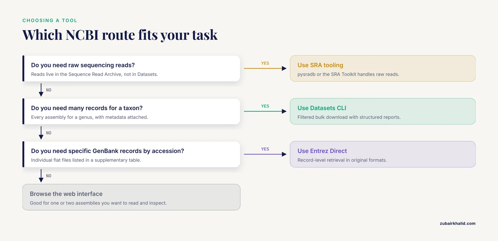
Before committing to any single tool, it helps to understand where the Datasets command-line interface sits among the other ways to pull data out of NCBI. Choosing the wrong route is one of the quiet time sinks in bioinformatics work: people spend hours scripting around a tool that was never designed for their query shape.
The NCBI web interface is optimized for human browsing. You search, you read, you click through to a record, and you download one file at a time. That is the right mode when you are exploring an unfamiliar organism, reading an assembly's annotation summary, or deciding which genome to feature in a figure. It is the wrong mode the moment a task involves more than a handful of records, because every click is manual labor that cannot be versioned or repeated.
The Datasets command-line tool is optimized for coherent packages. It returns assemblies, genes, taxonomy nodes, and ortholog sets as self-contained archives that bundle sequences with structured metadata reports [1]. This packaging philosophy is the tool's defining trait: rather than handing you a FASTA file and expecting you to reconstruct the context later, it hands you the sequences and the machine-readable context together.
Entrez Direct occupies a different niche. It speaks the full Entrez query language across essentially all NCBI databases, which means it can do things Datasets cannot, such as fetch individual flat-file GenBank records by accession, walk link sets between databases, or pull literature records. The tradeoff is that you assemble the context yourself. If your task is "give me 4,000 individual GenBank records listed in a supplementary table," Entrez Direct or Efetch is the better fit, and it largely replaces what people once did with the graphical NCBI Mass Sequence Downloader [8]. If your task is "give me every complete genome for this genus with its metadata," Datasets is decisively better.
A simple decision table:
| Task shape | Best first tool | Why |
|---|---|---|
| - | - | - |
| One or two assemblies, for reading and inspection | Web interface | Human-readable annotation summaries, no setup |
| Every assembly for a taxon, with metadata | Datasets CLI | Filtered bulk download with structured reports |
| Specific GenBank records by accession, flat files | Entrez Direct / Efetch | Record-level retrieval in original formats |
| Gene orthologs across species | Datasets CLI | Direct exposure of the NCBI Orthologs assignments [2] |
| Raw sequencing reads | SRA tooling such as pysradb | Reads are outside the Datasets domains [4] |
| TaxId lineage surgery at scale | TaxonKit alongside Datasets | Specialized taxonomy manipulation [5] |
A practical habit is to treat Datasets as your default for genome and gene acquisition, and to reach for the other tools only when your query shape falls outside its domains. Mixing tools is normal; the failure mode is assuming one tool covers everything.
Inside a Data Package: Reading the Manifest and Reports Like a Native
The draft walked through the directory layout briefly. This section goes deeper, because the quality of everything downstream depends on how well you understand what is actually inside the zip.
Every package contains three kinds of content: the data files you requested, one or more JSON report files, and the manifest. When you unzip a package, resist the urge to jump straight to the FASTA. Open the catalog first:
unzip -l listeria.zip | head -30This lists every file with its size before you extract anything, which is a cheap way to confirm the package matches your expectations. After extraction, read the manifest:
cat listeria/ncbi_dataset/data/dataset_catalog.jsonThe catalog is a JSON description of the package contents. The single most useful scripting pattern is to derive file paths from it rather than hardcoding them:
GENOME_FASTA=$(jq -r '.. | objects | select(has("path")) | .path' \
  listeria/ncbi_dataset/data/dataset_catalog.json \
  | grep "genomic.fna$" | head -1)
The precise key names inside the catalog can vary between tool versions, so treat this command as an exploratory template: run jq '.' dataset_catalog.json once to see the actual structure in your version, then adapt the filter. This exploratory-first habit protects you against the layout drift that the draft's common-mistakes section warns about.
The report files deserve their own explanation. assembly_data_report.jsonl holds one JSON object per line, each describing one assembly. To see the top-level structure of a single record:
head -1 listeria/ncbi_dataset/data/assembly_data_report.jsonl | jq 'keys'This tells you what the report contains in your installed version without guessing. Typical top-level groupings describe the organism, the assembly statistics, and the annotation status. You never need to parse these files by hand in production work; dataformat exists precisely to flatten them. But knowing the structure matters when you debug a conversion, when a field you expected is absent for a particular assembly, or when you want a piece of metadata that no TSV field exposes.
One subtlety worth internalizing: the reports describe only what the package contains, not everything NCBI knows. If you download with -include genome,report and skip annotation files, the report still describes annotation status as a metadata field, but you will find no annotation files on disk. Mismatched expectations here generate confused support questions, so check your -include list whenever a file type seems missing.
A Deeper Dive into dataformat: Shaping Tables for Downstream Work
The draft showed one genome TSV conversion and one gene conversion. Since dataformat is the piece you will run most often after the first week, it deserves a fuller treatment.
The core mental model: dataformat reads a JSONL report and emits a table with one row per report record and one column per requested field. Field names are hierarchical, joined with hyphens, and version specific. Never type them from memory. Always confirm with:
dataformat tsv genome -helpThe help output lists the complete field vocabulary for the genome domain. The same pattern applies to dataformat tsv gene, dataformat tsv taxonomy, dataformat tsv ortholog, and the virus domain.
A richer gene table example, pulling identifiers that matter for downstream mapping:
dataformat tsv gene \
  -inputfile dmel-genes/ncbi_dataset/data/gene_data_report.jsonl \
  -fields gene-id,symbol,locus-tag,tax-id,tax-common-name,gene-type,description \
  -output-file dmel-genes.tsv
Once you have a TSV, ordinary Unix text tools become your analytics layer. Three patterns cover most needs.
Filtering rows by a column value:
awk -F'\t' 'NR==1 || $6=="protein-coding"' dmel-genes.tsv > pc-genes.tsvThis keeps the header and every row where the gene-type column equals protein-coding. Adjust the column index to match your field order.
Counting by category:
tail -n +2 dmel-genes.tsv | cut -f6 | sort | uniq -c | sort -rnThis produces a frequency table of gene types, which is a fast sanity check that your download returned what you think it returned.
Joining two tables on a shared key, for example a gene table and a taxonomy table both carrying tax-id:
sort -k4,4 genes.tsv > genes.sorted.tsv
sort -k1,1 taxa.tsv > taxa.sorted.tsv
join -t $'\t' -1 4 -2 1 genes.sorted.tsv taxa.sorted.tsv > genes-with-taxa.tsv
The join command requires both inputs sorted on the join columns, which the first two commands handle. This pattern is how you enrich gene metadata with full organism names and ranks without re-querying NCBI per record.
For collaborators, the spreadsheet output needs no extra work:
dataformat xlsx genome \
  -inputfile ecoli-ref/ncbi_dataset/data/assembly_data_report.jsonl \
  -fields accession,organism-name,assembly-level,assembly-stats-total-sequence-length \
  -output-file ecoli-assemblies.xlsx
Two cautions on output tables. First, some field values contain characters that surprise spreadsheet software, so spot-check the opening rows of any file you hand off. Second, TSV files with many columns become hard to read in a terminal; pipe through column -t -s $'\t' for inspection but always keep the raw tab-separated file as the artifact your scripts consume, since column-based pretty printing is for humans only.
Worked Project: Assembling a Quality-Controlled Genome Set for Pangenome Analysis
This section ties the pieces together into a realistic end-to-end task. Suppose you want to build a pangenome input set for a bacterial species: many assemblies, all reasonably complete, all annotated, all from RefSeq.
Phase 1: Survey with Summary
datasets summary genome taxon "Streptococcus agalactiae" \
  -assembly-source refseq \
  -assembly-level complete
Read the total count from the JSON output. This number determines your disk budget and whether the job needs an API key export first.
Phase 2: Download Metadata Only
Resist downloading sequences before you have decided which assemblies you want. A metadata-only pass is fast and cheap:
datasets download genome taxon "Streptococcus agalactiae" \
  -assembly-source refseq \
  -assembly-level complete \
  -include none \
  -filename sag-meta.zip
unzip -q sag-meta.zip -d sag-meta
Phase 3: Flatten and Filter
Convert the report to a working table with the fields that drive your quality decisions:
dataformat tsv genome \
  -inputfile sag-meta/ncbi_dataset/data/assembly_data_report.jsonl \
  -fields accession,organism-name,assembly-level,assembly-stats-contig-n50,assembly-stats-total-sequence-length,annotation-provider \
  -output-file sag-all.tsv
Now filter. The thresholds here are illustrative choices for the example, not universal standards; pick values appropriate to your organism and question:
awk -F'\t' 'NR==1 {print; next}
  $4 >= 100000 && $5 >= 1800000 && $6 != "" {print $1}' \
  sag-all.tsv | tail -n +2 > sag-keep.txt
This keeps assemblies whose contig N50 is at least 100 kilobases, whose total length is at least roughly the expected genome size for the species, and which carry annotation from some provider. Inspect the counts at each step:
wc -l sag-keep.txtIf the filter is more aggressive than you intended, loosen a threshold and rerun. This is exactly why the metadata-only pass exists: iteration costs seconds, not gigabytes.
Phase 4: Fetch Sequences for the Survivors
Pass the filtered accession list back to Datasets:
datasets download genome accession \
  -inputfile sag-keep.txt \
  -include genome,gff3,protein,report \
  -filename sag-pan.zip
Unzip, and you have a directory tree where each assembly's FASTA sits next to its GFF3 and protein files, which is the input layout most pangenome and annotation pipelines expect. Because the two-pass design separates selection from retrieval, you can rerun Phase 4 with a corrected filter list without paying for metadata downloads again, and you can archive sag-all.tsv and sag-keep.txt as the record of exactly how your input set was defined.
This two-pass pattern, metadata first and sequences second, generalizes far beyond pangenomes. Any time selection criteria are uncertain, do the cheap pass first.
Large-Job Strategies: API Keys, Dry Runs, and the Dehydrated Pattern
Taxon-wide downloads of a few dozen assemblies are trivial. Downloads of tens of thousands are a different operational category, and a few strategies separate them.
First, always export the API key before a large job. Without a key your session shares anonymous request limits with everyone else, and the symptom is not usually an error but slow, halting progress on a job you expected to finish quickly.
Second, treat -dry-run as mandatory planning infrastructure for large selections. It previews the chosen records and the files that would be retrieved, which lets you estimate disk usage before committing. A genus with tens of thousands of assemblies, requested with full contents, can exceed expectations dramatically because protein and annotation files multiply the footprint of every assembly.
Third, recent versions of the tool support a dehydrated download pattern designed for exactly the large-job case. In this two-step flow, the initial download fetches the package structure and reports without the sequence payloads, you can inspect and even subset the package, and a rehydration step then fills in the sequence files. Check your installed version's help before relying on it, since the option appeared in later releases:
datasets download genome -help | grep -i dehydratIf your version supports it, the pattern looks like this in outline: download with the dehydrated flag, unzip as usual, inspect the reports and catalog, then run the rehydrate subcommand pointing at the extracted directory to fill in the sequences. This is particularly valuable on clusters where the filesystem where you inspect the package may not be the filesystem where you ultimately want the bulk sequence data, and it pairs naturally with the accession-list workflow from the worked project: dehydrate, decide, rehydrate only what survives your filters.
Fourth, serialize deliberately. Running many Datasets downloads in tight parallel loops against NCBI is poor citizenship and, without an API key, counterproductive. If you need many independent small packages, a modest degree of parallelism with the key exported behaves far better than an unthrottled fan-out.
Finally, log everything. A timestamped log line per download, recording the full command and the exit status, converts a mystery six weeks later into a one-line answer.
Scripting Patterns: Loops, Exit Codes, and Idempotent Pipelines
The draft's Step 8 showed a single-taxon script. Real projects usually involve loops over taxa or repeated monthly runs, and shell scripting around Datasets has a few patterns worth standardizing.
An idempotent loop that skips already-completed taxa:
#!/bin/bash
set -euo pipefail

for TAXON in "Listeria monocytogenes" "Bacillus subtilis" "Enterococcus faecalis"; do
  SAFE=$(echo "$TAXON" | tr ' ' '_')
  OUT="${SAFE}_$(date +%Y-%m-%d)"
  if [[ -d "$OUT" ]]; then
    echo "SKIP $TAXON (exists)"
    continue
  fi
  datasets download genome taxon "$TAXON" \
    -reference -include genome,gbff,report \
    -filename "${OUT}.zip"
  unzip -q "${OUT}.zip" -d "$OUT"
  echo "OK $TAXON $(date -Iseconds)" >> download.log
done
Three details earn their place here. The set -euo pipefail line makes the script fail loudly on the first error instead of continuing with a missing package, which prevents the worst failure mode: downstream steps silently consuming yesterday's data because today's download failed. The directory existence check makes reruns cheap and safe, so a cron job or a manually restarted batch does not refetch completed taxa. And the log line appends a machine-readable completion record, which pairs with the provenance practices below.
Checksum every zip you intend to keep:
sha256sum *.zip > checksums.sha256The checksum file is tiny, but it is the difference between "I think this is the archive I downloaded in March" and a verifiable statement. Verify later with sha256sum -c checksums.sha256.
When a loop step fails, capture the failing command explicitly rather than letting the error scroll past:
if ! datasets download genome taxon "$TAXON" -reference \
     -include genome,report -filename "${OUT}.zip"; then
  echo "FAIL $TAXON" >> download.log
  exit 1
fi
A batch that stops at its first failure with a clean log is far easier to resume than a batch that limped through half its taxa with silent gaps.
Going Further with Taxonomy: Lineage Tables and Classifier Inputs
The draft introduced the taxonomy domain. Two deeper applications justify more attention, because taxonomy identifiers are the glue that connects almost every other dataset you will handle.
The first application is building a lineage table for a subtree. A package downloaded with the tree, ids, and name reports gives you classification structure for every node under your query taxon. Flatten it:
dataformat tsv taxonomy \
  -inputfile bombus-tax/ncbi_dataset/data/taxon_data_report.jsonl \
  -fields tax-id,tax-common-name,formal-name,rank,genetic-code \
  -output-file bombus.tsv
The tax-id column is your stable join key. Nearly every NCBI-derived table you generate, whether from the genome domain, the gene domain, or an annotation pipeline's output, can be joined back to this table on tax-id. Build the lineage table once for your project's organisms and reuse it everywhere.
The second application is feeding downstream classification tools. Metagenomic profilers and lowest-common-ancestor tools generally want NCBI taxonomy in their own preferred formats. Rather than hand-crafting those formats, combine tools along their strengths: Datasets retrieves the subtree and its identifiers, TaxonKit performs fast TaxId operations and lineage reformatting on the taxonomy dump with its dedicated subcommands [5], and a profiler such as ngsLCA consumes NCBI taxonomy inputs directly for LCA-style read assignment. The Datasets taxonomy domain gives you the curated, current view of names and classification that NCBI maintains, and its programmatic access expanded notably when NCBI broadened taxonomy availability across APIs and command-line surfaces in 2024 [3].
One practical warning: taxon names are not identifiers. Synonyms, spelling variants, and name changes mean that string matching on organism names is fragile across time. Wherever a pipeline allows it, carry tax-id, not the name, as the key, and resolve names to identifiers once, at the boundary of your workflow, rather than repeatedly deep inside it.
Troubleshooting Field Guide: Symptoms, Causes, Fixes
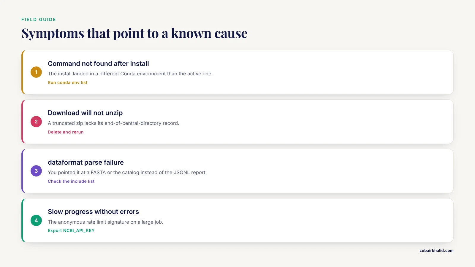
The draft's common-mistakes list covers query-construction errors. This section addresses the operational and environment problems that surface once you are past your first commands.
Command not found immediately after installing. If datasets -version fails right after a Conda install, the almost universal cause is that the install landed in a different environment than the one currently active. Run conda env list, activate the environment you installed into explicitly, and retry. This single diagnosis resolves a large share of first-day failures.
A download that completed but will not unzip. A zip truncated by an interrupted connection lacks its end-of-central-directory record and refuses to open. The draft noted the error text; the operational fix is to make retries routine. Delete the partial file, rerun the download, and if the job is large enough that interruptions are likely, prefer the dehydrated pattern, which reduces the payload of the vulnerable first step.
dataformat complains about its input file. Passing a FASTA or a catalog JSON where a JSONL report is expected produces a parse failure. The reports end in .jsonl and live alongside the data directory; the catalog is a single JSON object. Confirm you are pointing at the right file, and confirm the package actually contains a report by checking your original -include list, since requesting none for the report type yields no report to convert.
A summary returns zero records for an organism you know exists. Taxon-name resolution is doing more work than you think. Try the TaxId directly, try the genus name alone, and check spelling. NCBI Taxonomy includes synonyms, but your string must match something in that index. This is the same fragility discussed in the taxonomy section, and the same cure applies: resolve once to an identifier, then use the identifier.
Slow, halting progress on a large job without errors. This is the anonymous-rate-limit signature. Export your API key, confirm it is visible with echo $NCBI_API_KEY in the same shell, and rerun. If you are scripting across many shells or a scheduler, set the variable in the job environment, not only in your interactive profile.
Field value missing for some rows in a converted table. Not every assembly carries every field. Unannotated assemblies have nothing for annotation-provider fields; infraspecific names are absent when the submitter supplied none. Empty cells are normal, not corruption. Design filters to treat empty annotation fields explicitly rather than assuming every row is fully populated.
Weird behavior with taxon names containing spaces in scripts. Unquoted or partially quoted variables expand into multiple arguments. Quote every variable expansion in scripts: "$TAXON", not $TAXON. This is elementary shell hygiene, but it is the root cause behind many "unable to parse taxon" reports that appear only inside scripts and never at the interactive prompt.
Common Misconceptions About NCBI Access
Several beliefs circulate that cost people real time. Correcting them explicitly is faster than discovering each by failure.
Misconception: Datasets replaces all other NCBI programmatic access. It covers assemblies, genes, taxonomy summaries, orthologs, and SARS-CoV-2 viral data. It does not cover raw reads, individual legacy record formats across all databases, literature, or arbitrary Entrez link walks. A realistic NCBI toolkit keeps Entrez Direct and SRA-specific tooling such as pysradb alongside Datasets [4].
Misconception: the reference flag means the best assembly for a genus. Reference status is designated per species, and asking for the references of a genus returns one assembly per species in that genus, not one total. If you want a single representative for a higher taxon, you need to make that selection yourself from a filtered table.
Misconception: GenBank assemblies are unreliable and RefSeq assemblies are the only usable ones. RefSeq assemblies receive NCBI-mediated curation and verification, which makes them the sensible default when you need one well-behaved genome per organism. But GenBank is the archive of record, and for many organisms the only available assemblies are GenBank-only. The honest framing is that assembly-source selection is a question about your tolerance for heterogeneity, not a binary quality verdict.
Misconception: ortholog assignments are simple reciprocal best hits. The NCBI Orthologs pipeline computes relationships through its own pipeline and integrates them into the Gene resource, and the Datasets ortholog endpoint exposes those assignments [2]. The ortholog-category field in the report distinguishes relationship types. Read it rather than assuming every row means a one-to-one equivalence.
Misconception: what I downloaded today is what I will download next year. NCBI content evolves continuously, accessions get new versions, and assemblies get replaced or suppressed. Sequence database versioning is a recognized reproducibility problem precisely because pipelines rerun months apart encounter different reference content [6]. Archive your packages locally and record versions; do not treat NCBI as your long-term storage.
Misconception: the zip contains everything about an assembly. It contains what your -include list and filters selected, plus the reports. Structural annotation, functional annotation, expression data, and literature links are not implicitly bundled. Read the catalog to know what you hold.
Practical Application Recipes
Brief recipes for tasks that recur across projects.
Marker protein set for phylogenetics. Pick a conserved gene, find its GeneID, then pull its ortholog set across taxa with the ortholog endpoint. The package's protein FASTA files give you one protein per organism, and the flattened report gives you the species mapping you need to label sequences for alignment and tree building [2].
Reference panel refresh. For a monthly-updated reference set, script the summary, filter with -released-since set to your last refresh date, and append only new assemblies to your existing local collection. This incremental pattern keeps a maintained panel current without refetching everything, and it pairs naturally with the version-recording discipline [6].
Teaching subset. For a classroom exercise, download the reference genomes of five well-known organisms with metadata-only plus genome, flatten to a spreadsheet with dataformat xlsx, and hand students a curated, self-contained package. Students get real NCBI data with no browsing overhead, and you get a reproducible exercise definition.
Annotation pipeline inputs. Most prokaryotic annotation workflows and genome browsers accept a genomic FASTA plus GFF3, both of which come straight from the genome package. When a specific downstream schema demands something unusual, check before assuming; for instance, NCBI .tbl feature tables require conversion for certain UCSC-format destinations, and purpose-built parsers exist for that case [7].
Cross-domain join for meta-analysis. Download a gene package for a taxon, download a taxonomy lineage table for the same clade, and join on tax-id using the sort-and-join pattern shown earlier. The result is a single table where every gene row carries full organism context, ready for filtering or plotting.
Provenance, Archiving, and Sharing Your Downloads
Reproducibility with NCBI data is an archiving discipline, not a promise. Because the underlying databases change continuously, the artifact you can defend is not "the E. coli genome" but "this specific package, retrieved by this specific tool version on this date" [6].
Concretely, every project directory that consumed Datasets data should contain four things. First, the packages themselves, or at minimum their checksums and the small report files, if storage constraints force you to discard sequences. Second, checksums.sha256 for everything retained. Third, a plain-text manifest recording the tool version from datasets -version, the download dates, and the exact commands run, which is easiest to generate by writing your download commands into a script and treating the script as the manifest. Fourth, the dataset_catalog.json from every package, since the catalog enumerates exactly which files the package was supposed to contain and lets a future reader verify completeness without the archive present.
For team settings, wrap the tool in an environment specification so colleagues reconstruct your toolchain rather than a similar one:
# environment.yml
name: ncbi-datasets
dependencies:
  - conda-forge::ncbi-datasets-cli
Anyone can then rebuild the same retrieval environment with conda env create -f environment.yml. Combined with the checksums and the catalog files, this closes the loop: the data state, the tool state, and the commands are all recorded, and the record is verifiable rather than anecdotal. The FAIR packaging design that motivated the Datasets resource extends naturally to your side of the transaction; the package you archive is findable, self-describing, and reusable exactly because it carried its context with it from the start [1].
Frequently Asked Questions
What is the difference between the datasets and dataformat commands?
datasets queries NCBI and downloads zip data packages, while dataformat converts the JSON reports inside those packages into TSV, CSV, or XLSX tables. You almost always use them in sequence: download with datasets, then flatten with dataformat.
How do I install the NCBI Datasets command-line tool?
Run conda install -c conda-forge ncbi-datasets-cli, or download a prebuilt binary for your platform from the NCBI datasets command-line directory on the NCBI public FTP site. Verify with datasets, version.
How do I download only reference genomes for a species?
Add -reference to a genome download, for example datasets download genome taxon "Escherichia coli", reference. This returns the single designated reference assembly rather than every assembly for the species.
Can the tool download raw sequencing reads from the SRA?
No. The Datasets tools cover assemblies, genes, taxonomy, and orthologs, not raw read data. Use a dedicated SRA tool such as pysradb, which provides command-line querying and downloading of SRA metadata and reads [4].
How do I find the full list of fields for a TSV conversion?
Run the help for the specific subcommand, for example dataformat tsv genome, help, which prints the complete field vocabulary. Field names are hierarchical and version specific, so copy them from help output rather than guessing.
How do I retrieve the orthologs of a human gene?
Use the ortholog selector, for example datasets download gene ortholog 672, include protein. GeneID 672 corresponds to human BRCA1, and the returned package contains each ortholog with its species, symbol, and ortholog category as computed by the NCBI Orthologs pipeline [2].
Do I need an NCBI API key to use the tools?
No, the tools work without one for routine queries. For large or frequent downloads, export your key as the NCBI_API_KEY environment variable so the service applies higher request limits to your session.
How do I record exactly what I downloaded for reproducibility?
Save the tool version from datasets, version, the download date, and the dataset_catalog.json file from every package. NCBI content changes continuously, so these three artifacts are what let you reconstruct the exact dataset state months later [6].
Sources
- Exploring and retrieving sequence and metadata for species across the tree of life with NCBI Datasets
- NCBI Orthologs: Public Resource and Scalable Method for Computing High-Precision Orthologs Across Eukaryotic Genomes
- NCBI taxonomy: enhanced access via NCBI datasets.
- pysradb: A Python package to query next-generation sequencing metadata and data from NCBI Sequence Read Archive
- TaxonKit: A practical and efficient NCBI taxonomy toolkit.
- Sequence database versioning for command line and Galaxy bioinformatics servers
- Tbl2KnownGene: A command-line program to convert NCBI.tbl to UCSC knownGene.txt data file
- NCBI Mass Sequence Downloader-Large dataset downloading made easy