Resolving Low Mapping Rates in RNA-seq

By Dr. Zubair Khalid, DVM, MS, PhD · 2026-11-11

After working through this article you will be able to do four things with a poorly mapping RNA-seq sample. First, you will extract the exact mapping statistics from an alignment log and interpret each category of unmapped read. Second, you will run a systematic diagnostic sequence that separates read-quality problems from reference problems from parameter problems. Third, you will re-run the alignment with corrected settings and confirm the fix with independent checks. Fourth, you will recognize the cases where a low mapping rate reflects the biological material or the organism, not a mistake on your part.

Before you start, install and test these tools on your system: a splice-aware aligner (STAR or HISAT2), samtools, FastQC, MultiQC, cutadapt, and a terminal with at least 32 GB of RAM available for building a mammalian genome index. All commands below assume a Unix shell and paired-end data in FASTQ format.

What Counts as a Low Mapping Rate in RNA-seq

Context matters before you change anything. In a controlled pipeline comparison on human samples, STAR mapped 98.98 percent of reads from a Burkitt lymphoma cell line dataset and 98.49 percent of reads from a rectal cancer patient dataset, while TopHat2 reached 97.02 and 96.73 percent on the same data [1]. A specialized low-input protocol reported a mapping ratio of approximately 90 percent with duplication no higher than 25 percent [2]. In a veterinary dataset against the feline genome, thirteen RNA-seq libraries showed similar duplication and mapping rates of 94 to 95 percent despite varying RNA quality [3].

A practical working rule for well-annotated model organisms with high-quality RNA: a uniquely mapped fraction below about 80 percent deserves investigation, and a total mapped fraction below about 70 percent signals a real problem. For organisms with a distant or absent reference genome, or for material rich in repetitive sequence, lower rates can be normal. The classification step below tells you which situation you are in.

Bioinformatics troubleshooting works best when you change one variable at a time. Each step below isolates one hypothesis.

A Step-by-Step Diagnostic Workflow for Low Mapping Rate RNA-seq

Step 1. Read the Aligner Log Before Touching Anything Else

If you aligned with STAR, open Log.final.out in the output prefix directory. This file already splits your unmapped reads into the categories that matter.

grep -E "Number of input reads|Uniquely mapped|multiple loci|too many loci|too short|other" sample/Log.final.out

Expected output from a healthy mammalian sample looks like this:

Number of input reads |	25000000
Uniquely mapped reads number |	23225000
Uniquely mapped reads % |	92.90%
% of reads mapped to multiple loci |	2.10%
% of reads mapped to too many loci |	0.60%
% of reads unmapped: too short a match |	3.90%
% of reads unmapped: other |	0.50%

If you used HISAT2, request the summary explicitly the next time, because it is not written by default:

hisat2 -x hg38_hisat2_index -1 R1.fastq.gz -2 R2.fastq.gz \
  --summary-file sample_hisat2_summary.txt -S sample.sam

A cross-pipeline comparison of four RNA-seq pipelines on the same matched datasets found that aligner choice alone changed overall mapping rate dramatically, from 98.98 percent for STAR down to 54.44 percent for Sailfish on the patient dataset [1]. This is why the aligner log, not a generic sense that the number looks low, must drive the diagnosis.

For a quick independent count from the BAM file itself, run:

samtools flagstat sample_Aligned.sortedByCoord.out.bam

Expected output:

25000000 + 0 in total (QC-passed reads + QC-failed reads)
23700000 + 0 primary mapped (94.80% : N/A)

The percentages from flagstat and the aligner log should agree within rounding. If they disagree wildly, you are probably comparing a filtered BAM against unfiltered input, which is one of the quietest sources of a false low mapping rate.

Step 2. Classify the Unmapped Reads

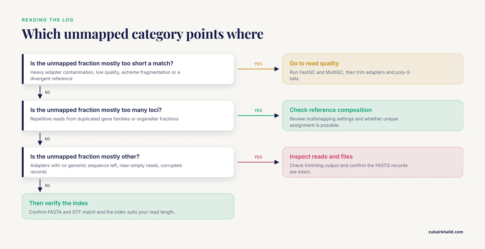
Each STAR category points to a different root cause:

• Unmapped, too many loci. The reads are repetitive. Expect this from organisms with large duplicated gene families, from samples with organellar or transposon-rich fractions, and from certain library types. This category is often not an error at all.
• Unmapped, too short a match. The aligner could not find a long enough anchored seed on the genome. Causes include heavy adapter contamination, low sequence quality, extreme fragmentation of the input RNA, or a reference genome too divergent from your sample.
• Unmapped, other. Typically adapters without enough genomic sequence left over, near-empty reads after trimming, or corrupted records.

The ratio between these categories is your first fork in the diagnostic road. A profile dominated by "too short" sends you toward read quality and trimming. A profile dominated by "too many loci" sends you toward reference composition and multimapping settings.

Step 3. Inspect Read Quality and Composition with FastQC and MultiQC

fastqc -t 8 -o qc/ *.fastq.gz
multiqc qc/ -o qc/multiqc_report

Open the MultiQC report and check four modules in this order.

1. Adapter Content. Rising adapter curves at the read ends mean untrimmed libraries. Adapter sequence at the read start or full-read adapter means inserts shorter than the read length.
2. Per base sequence quality. Falling quality toward the 3-prime end is normal for longer reads. Quality collapsing early in the read points to sequencing problems.
3. Overrepresented sequences. Runs of a single sequence at high abundance often indicate rRNA or other abundant transcripts, which is a composition problem rather than a quality problem.
4. Per tile quality and poly-G signals. On two-color chemistry instruments such as NextSeq and NovaSeq, failing to call a base produces poly-G tails that read as high-quality G stretches and inflate mismatch counts. Cutadapt handles this directly (Step 6).

Step 4. Check for Dominant Off-Target Fractions

A library that is mostly rRNA can align beautifully to the genome yet waste most of its depth. Library preparation strategy changes what maps where. In a study comparing three library strategies on leaf RNA from the medicinal plant Glycyrrhiza uralensis, rRNA-depleted libraries produced numerous rRNA-linked artifacts, total RNA-seq detected the most genuine plastid RNA editing sites, and mRNA-seq libraries showed very low plastid mapping rates even though targeted, strand-aware analysis still recovered a large fraction of bona fide sites [4]. The lesson generalizes: the expected on-target fraction differs by protocol, and a low rate against one compartment can coexist with a fine library for its intended compartment.

If contamination by another organism is plausible, screen a subsample of reads against a panel of candidate references. Tools such as Kraken2 or FastQ Screen classify reads by source organism, and a 100,000-read subsample is enough to reveal a dominant contaminant without a full run.

Step 5. Verify the Reference Genome and the Index

Reference mismatch is the most common cause of a catastrophic, sample-wide mapping collapse, and it is also the easiest to check.

Confirm three things before realigning:

1. The FASTA and the annotation match. A GTF from one assembly release aligned against a FASTA from another produces silent chaos. Download both from the same source and record the release identifiers.
2. The index was built for your read length. STAR indices store the splice junction database with a read-length-dependent parameter, so an index built for 100-base reads performs poorly on 150-base reads. The relevant parameter at index build time is -sjdbOverhang, which should be your read length minus one.
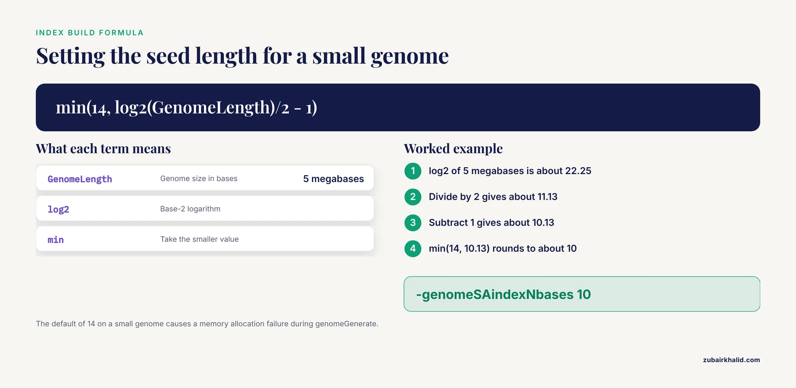
3. The index suits your genome size. The suffix-array seed length parameter -genomeSAindexNbases should be min(14, log2(GenomeLength)/2 - 1). For a 5-megabase bacterial genome, that computes to about 10, not the default 14. Using 14 on a small genome produces the well-known memory error described in the next section.

A correct genome index build for paired-end 150-base human reads looks like this:

STAR --runMode genomeGenerate \
  --genomeDir hg38_star_index \
  --genomeFastaFiles hg38.fa \
  --sjdbGTFfile gencode.annotation.gtf \
  --sjdbOverhang 149 \
  --genomeSAindexNbases 14 \
  --runThreadN 16

STAR was developed specifically to handle the non-contiguous structure of transcripts against a genomic reference, and it detects both canonical and non-canonical splice junctions along with chimeric transcripts [5]. Those junction-aware capabilities are exactly what a correctly built index unlocks.

Step 6. Trim Adapters and Poly-G Tails

For standard Illumina adapters:

cutadapt -a AGATCGGAAGAGCACACGTCTGAACTCCAGTCA \
         -A AGATCGGAAGAGCACACGTCTGAACTCCAGTCA \
         -m 30 -q 20 \
         -o R1.trim.fastq.gz -p R2.trim.fastq.gz \
         R1.fastq.gz R2.fastq.gz

For NovaSeq or NextSeq data, add the poly-G trimmer:

cutadapt --nextseq-trim=20 -a AGATCGGAAGAGC -A AGATCGGAAGAGC \
         -m 30 -o R1.trim.fastq.gz -p R2.trim.fastq.gz \
         R1.fastq.gz R2.fastq.gz

Expected cutadapt output:

Total basepairs processed: 15,200,000,000 bp
  Read 1 with adapter: 812,345 (6.5%)
Pairs written (passing filters): 11,900,000 (95.20%)

Use the gentlest trim that fixes the problem. The minimum length filter of 30 bases keeps fragments short enough for degraded samples while discarding adapter-only reads.

Step 7. Realign with Corrected Parameters

The core STAR alignment command:

STAR --runThreadN 16 \
  --genomeDir hg38_star_index \
  --readFilesIn R1.trim.fastq.gz R2.trim.fastq.gz \
  --readFilesCommand zcat \
  --outFileNamePrefix sample_ \
  --outSAMtype BAM SortedByCoordinate \
  --twopassMode Basic \
  --outFilterMultimapNmax 10 \
  --outFilterMismatchNmax 10

The parameters that matter most:

Two warnings about loosening filters. Raising mismatch tolerance recovers genuinely fragmented reads but also admits spurious alignments, and aligner documentation stresses that mismatch filtering protects specificity. Any gain in rate from loosened filters should be checked against the quality checks in the verification section.

Step 8. Cross-Check with a Second Aligner

When the numbers stay stubbornly low with clean data and a verified index, try HISAT2 and compare:

hisat2 -x hg38_hisat2_index \
  -1 R1.trim.fastq.gz -2 R2.trim.fastq.gz \
  --summary-file sample_hisat2_summary.txt \
  -S sample_hisat2.sam

Expected HISAT2 summary:

25000000 reads; of these:
  25000000 (100.00%) were paired; of these:
    24125000 (96.50%) aligned concordantly 0 times

HISAT2 and STAR use different seed-search strategies, so a sample that aligns at 85 percent with one and 92 percent with the other is telling you where the reads are hard to place. Keep in mind that a comparison study found real rate differences between pipelines even on the same human samples, so the second aligner is a probe, not necessarily the final choice [1].

Step 9. Verify That the Fixed Alignment Is Actually Right

A higher mapping rate is only good news if the mapping is correct. Run these checks on every revised alignment:

1. Spot-check read origins in IGV. Open a handful of highly expressed genes and confirm that reads pile up on exons in the expected orientation. Visual verification in IGV was part of the stringent filtering workflow in the plastid editing study cited above [4].
2. Confirm strandness. Run RSeQC infer_experiment.py on the BAM and confirm the inferred library type matches the kit you used. A strandness mismatch silently halves apparent sense mapping.
3. Check duplication and library complexity. High duplication with a high mapping rate can mean PCR overamplification rather than success. The feline tooth study found that one low-yield sample with otherwise good RNA showed elevated duplication, a warning that yield and complexity interact [3].
4. Validate a few expression signals externally. Downstream differential expression calls in published RNA-seq studies are commonly validated by RT-qPCR on selected genes, which is the standard way to confirm that the pipeline is measuring real biology rather than alignment artifacts [8].

Common Errors, Exact Messages, and Fixes

STAR exits during genomeGenerate with a memory allocation failure. When the genome is small and -genomeSAindexNbases stays at the default 14, STAR fails with an allocation error and exits before writing an index. Fix: recompute the parameter with the formula min(14, log2(GenomeLength)/2 - 1) and rebuild.

STAR reports essentially zero mapped reads with a FASTQ parsing complaint. The usual cause is gzipped input without -readFilesCommand zcat, so STAR reads compressed bytes as sequence. Fix: either add the flag or point -readFilesIn at decompressed files. The same symptom appears if the FASTQ files are truncated or are actually FASTA files.

samtools refuses the BAM file. The message [E::hts_open_format] Failed to open file means the path is wrong, the file is empty, or an earlier pipeline stage failed silently. Check the aligner log for the real failure before re-running samtools.

A shell reports unrecognized option for an aligner flag. Splice-aware aligners differ in flag syntax, and flags valid for one tool or version fail on another. Run the tool with -help under the exact version you have installed rather than copying flags from a tutorial written for a different release.

MultiQC shows per-sample mapping rates that look scrambled. The most frequent cause is a metadata mismatch, where file names with swapped sample labels were renamed or copied out of order during demultiplexing. Mapping statistics travel with the file, so if sample A consistently maps to an unrelated fraction, suspect that the file carries the wrong label, not that the library is wrong.

Special Cases That Change What "Low" Means

Degraded and Low-Input RNA

Some tissues deliver fragmented RNA no matter what the lab does. Spermatozoa, for example, carry very small amounts of highly fragmented RNA, and the boar sperm RNA-seq literature treats purification, extraction, and kit choice as the deciding factors for whether sequencing works at all [9]. Single-embryo work pushes inputs even lower, and dedicated low-input protocols are built around the expectation that raw mapping fractions will be lower than bulk tissue [10]. In those settings, a mapping rate that would be alarming for liver tissue may be the realistic ceiling for the material, and the appropriate response is a protocol matched to the input rather than a longer list of alignment flags.

One counterintuitive finding is worth knowing before you discard a batch on quality grounds. The feline tooth extraction study measured RNA integrity with an RINe equivalent and found that thirteen RNA-seq libraries produced similar duplication and mapping rates of 94 to 95 percent regardless of RINe values, meaning moderate degradation did not hurt mapping [3]. The same study found that A260:280 and A260:230 purity ratios did not correlate with degradation, so purity ratios are unreliable proxies for integrity. Degradation matters most for fragment-length-sensitive quantification, not always for raw mapping.

Non-Model Organisms Without a Reference

If your species has no assembled genome, a low mapping rate against a relative's genome is expected rather than pathological. Two standard paths exist. The first is de novo transcriptome assembly from your own reads using assemblers such as Trinity, SOAPdenovo-Trans, or TransABySS, then remapping raw reads against the assembly. In the peanut transcriptome study, assemblies from all three assemblers reached N50 values between roughly 1100 and 1650 base pairs and contained more than 40 percent full-length transcripts, giving usable reference targets for non-model species [11]. The second path is read classification against multiple reference sets. For the parasitic plant Cuscuta on its host Impatiens, researchers without a reference genome classified RNA-seq reads as host or parasite by stepwise similarity searches against de novo assembled transcript sets from both organisms [12]. That same approach solves any project where reads from two genomes are mixed and neither maps cleanly against the other's reference alone.

Divergent Genomes and Individual Variants

Even with a reference for your species, individual variation creates unmappable reads. Sequence variants that create novel splice site dinucleotides generate junction reads that standard aligners, which rely on consensus splice motifs against the reference, cannot place. Mapping personal transcriptomes against personal genomes recovered this hidden variation, identifying 506 personal-specific splice junctions in a cohort of 75 individuals, of which 437 were absent from existing annotations [13]. For SNP-tolerance and editing detection specifically, purpose-built aligners such as RASER reduce false-positive mappings in highly similar genomic regions where standard aligners misplace alternative alleles [7]. If your project involves divergent strains, outbred populations, or editing analysis, a fraction of unmapped reads is structural, and variant-aware mapping is the correct remedy.

Multimapping and Where the Counts Really Go

A read that maps to multiple loci is not lost, but its assignment is ambiguous, and quantification methods must split or discard it. This read mapping ambiguity is one of the two major difficulties in transcript quantification, alongside overdispersion of reads along the reference [6]. Fusion detection faces the same multiple-mapping problem, and specialized tools such as SOAPfusion were designed to handle multi-mapping reads while keeping false positives at or below about 1.4 percent [14]. When your low "uniquely mapped" number is really a high multimapping number, the fix is analytical rather than mechanical, and it starts with deciding whether the biology of your genes makes unique assignment possible at all.

Reads that land outside annotated exons are another gray zone. The XBSeq method was built on the observation that non-exonically mapped reads behave like measurable noise layered over true expression signals, and modeling them explicitly changed differential expression calls in evaluation datasets [15]. When you judge a mapping rate, decide consciously whether non-exonic and multimapping reads are waste to be discarded or signal to be modeled.

Sequencing Depth and Platform Context

Depth interacts with mapping statistics less directly than most people expect. Very deep samples do not inherently map better, but they expose small problematic fractions that shallow samples hide. For scale, a large pig placenta and endometrium RNA-seq data resource generated an average of 107 million reads per endometrial sample and 105 million per placental sample on the NovaSeq 6000 platform [16]. At that depth, even a 1 percent rRNA fraction represents a million reads, so compositional problems become visible and quantifiable. If your samples are much shallower and the mapping rate looks acceptable but the downstream counts look thin, the mapping rate was never the limiting problem.

Common Mistakes and Limitations

Blaming the aligner first. Aligner choice does move the number [1], but in practice the leading causes of a genuinely low mapping rate are reference mismatches, untrimmed adapters, and wrong-for-the-genome index settings. Realigning three times with three aligners before reading the log wastes more time than the log would have saved.

Aggressive trimming as a reflex. Trimming adapters is correct when the Adapter Content curve rises. Trimming quality bases off every read by default removes alignment anchors and can push borderline reads into the "too short" category, lowering the mapping rate you were trying to raise. Trim to the diagnosis, not to a habit.

Mixing assembly builds. A GTF from one release with a FASTA from another is the classic silent failure. Chromosome naming conventions that differ between sources, such as chr1 versus 1, compound the problem and can zero out an alignment run.

Reading purity ratios as integrity. Spectrophotometric ratios do not reliably reflect RNA integrity, as the feline tooth study demonstrated directly [3]. Use a gel- or capillary-based integrity measure and, ideally, a pilot sequencing run on one representative sample before committing a batch.

Expecting one mapping rate across library types. Total RNA-seq, rRNA-depleted, and mRNA-seq libraries target different compartments and produce systematically different organellar and rRNA fractions [4]. Comparing your mRNA-seq sample against a total RNA-seq benchmark produces false alarms.

Diagnosing from a single sample. A problem in one sample among twenty is a library problem. A problem in all twenty is a reference, index, or parameter problem. Check the pattern across samples before changing shared settings.

Treating unmapped reads as worthless. Non-exonic and multimapping reads carry information if you model them deliberately [15], and unmapped reads from divergent genomes can anchor personal splice discovery [13]. Disposal is a decision, not a default.

Confusing a low unique rate with a low total rate. Quantification pipelines tolerate multimappers differently, and a sample with 90 percent total mapping and 60 percent unique mapping may be perfectly usable for gene-level counting while unusable for allele-specific work. Name the number you care about before troubleshooting.

Finally, the general limitation: this workflow resolves computational and library-technical causes of low mapping rates. Persistent anomalies in expression patterns, in cross-contamination between samples, or in biological replicates require domain expertise about the organism and tissue in question, and a conversation with the sequencing provider or a collaborator who knows the material is the correct next step when the pipeline checks all come back clean.

Frequently Asked Questions

What is a good mapping rate for RNA-seq?

For model organisms with a high-quality reference, published pipelines commonly reach the mid-90s in percent, with STAR reporting 98.98 and 98.49 percent on two human datasets [1]. Below roughly 80 percent uniquely mapped, investigate. For non-model organisms, divergent strains, or fragmented input RNA, lower rates can be normal for the material.

What is the most common cause of a low mapping rate in RNA-seq?

A mismatch between the reads and the reference is the most common cause, meaning the wrong genome build, an index built with incompatible settings, or heavily contaminated reads. Check the aligner log categories and the index build parameters before trying alternative aligners, because those two checks resolve most cases in minutes.

Should I trim adapters before aligning?

Yes, when FastQC shows adapter contamination, because adapter sequence competes with genomic sequence for alignment. Trim with the shortest effective settings, keep a minimum-length filter around 30 bases, and add poly-G trimming on two-color instruments such as NextSeq and NovaSeq.

Can degraded RNA cause a low mapping rate?

Sometimes, but less often than commonly assumed. In one veterinary RNA-seq dataset, libraries from RNA spanning a range of measured integrity values all mapped at 94 to 95 percent [3]. Severe fragmentation does lower the rate and distorts fragment-based quantification, so match the library kit to the input rather than assuming degraded RNA automatically fails.

Why are so many of my reads mapping to rRNA?

The library preparation failed to deplete rRNA or was designed as total RNA-seq, where rRNA retention is expected. Library strategy changes the composition of what maps, and rRNA-depleted protocols in particular can produce rRNA-linked artifacts that strand-aware filtering must remove [4]. If rRNA dominates an mRNA-seq library, contact the sequencing provider about depletion efficiency.

Can I map RNA-seq reads to a related species' genome?

You can, and the mapping rate will be lower and biased toward conserved genes, which is acceptable for some analyses and misleading for others. For most non-model projects, de novo transcriptome assembly with tools such as Trinity followed by read remapping against your own assembly gives a more honest reference [11].

How do I handle reads that map to multiple locations?

Decide based on your question. For gene-level counting, standard quantifiers assign or discard multimappers according to defined rules, and the ambiguity is inherent to duplicated genes [6]. For allele-specific or editing analyses, use stricter settings or variant-aware alignment to keep only confident placements [7].

Which aligner gives better mapping rates, STAR or HISAT2?

Both are excellent, and the right answer is to measure on your own data. In a controlled comparison, STAR achieved the highest overall mapping rate of the pipelines tested [1], while HISAT2 offers comparable performance with different memory characteristics. If the two disagree by several percentage points on the same sample, that gap itself points to the cause.

Sources

1. A comparative study of RNA-Seq and microarray data analysis on the two examples of rectal-cancer patients and Burkitt Lymphoma cells.
2. Step-by-Step Protocol for In Situ Profiling of RNA Subcellular Localization Using TATA-seq.
3. Optimised isolation method for RNA extraction suitable for RNA sequencing from feline teeth collected in a clinical setting and at post mortem.
4. Plastid RNA Editing in Glycyrrhiza uralensis: Landscape Characterization and Comparative Assessment of RNA-Seq Library Strategies for Detection.
5. STAR: ultrafast universal RNA-seq aligner.
6. Modeling Exon-Specific Bias Distribution Improves the Analysis of RNA-Seq Data.
7. RASER: reads aligner for SNPs and editing sites of RNA.
8. RNA sequencing identifies transcriptional changes in the rabbit larynx in response to low humidity challenge.
9. A technical assessment of the porcine ejaculated spermatozoa for a sperm-specific RNA-seq analysis.
10. Mechanistic insights into HuR inhibitor MS-444 arresting embryonic development revealed by low-input RNA-seq and STORM.
11. Comparisons of de novo transcriptome assemblers in diploid and polyploid species using peanut (Arachis spp.) RNA-Seq data.
12. A bioinformatics approach to distinguish plant parasite and host transcriptomes in interface tissue by classifying RNA-Seq reads.
13. Discover hidden splicing variations by mapping personal transcriptomes to personal genomes.
14. SOAPfusion: a robust and effective computational fusion discovery tool for RNA-seq reads.
15. Differential expression analysis of RNA sequencing data by incorporating non-exonic mapped reads.
16. RNA-seq data of pig placenta and endometrium during late gestation.