How to Handle Large Single-Cell RNA-seq Data in R
By Dr. Zubair Khalid, DVM, MS, PhD ·

By the end of this guide you will be able to load a multi-million-cell single-cell RNA-seq experiment into R without filling your RAM, run memory-efficient dimension reduction and clustering, store intermediate objects on disk, and scale differential expression to cohort-level datasets. You will also know which common mistakes inflate memory use by an order of magnitude and how to check that each step actually worked.
Before you start, have the following ready:
- R 4.3 or later and RStudio (or any editor you like)
- Bioconductor installed, along with the packages used below:
SingleCellExperiment,scater,scran,DropletUtils,DelayedArray,HDF5Array,mbkmeans,irlba,BiocParallel - The
Matrixpackage (ships with R), and optionallySeuratif you work across ecosystems - HDF5 system libraries, which install automatically with
HDF5Arrayon Windows and macOS and through your package manager on Linux - A rough idea of your dataset size (cells, genes, and expected sparsity) so you can plan storage
Everything in this guide runs on a single workstation. If your machine has 32 to 64 GB of RAM, you can follow every step for datasets in the range of hundreds of thousands to about a million cells by keeping counts on disk.
Why Large Single-Cell RNA-seq Data Breaks Standard R Workflows
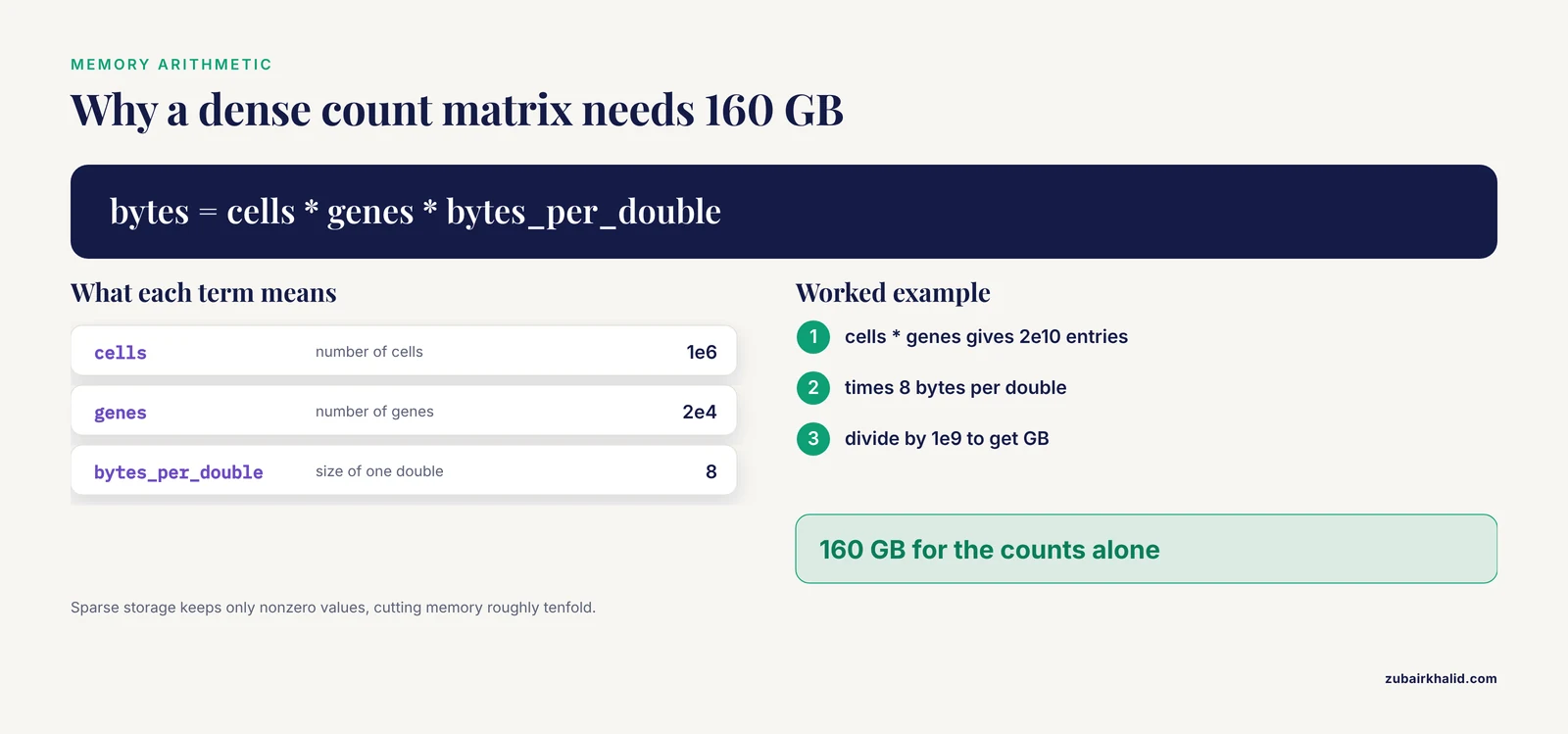
R keeps every object it creates in RAM. A raw count matrix from a single-cell experiment is mostly zeros, but if you store it as a standard dense matrix, R allocates memory for every zero. The arithmetic makes the problem concrete.
A dense double-precision matrix of 1 million cells by 20,000 genes needs:
cells <- 1e6
genes <- 2e4
bytes_per_double <- 8
bytes <- cells * genes * bytes_per_double
bytes / 1e9   # 160 GB
That is 160 GB for the counts alone, before normalization matrices, reduced dimensions, or metadata. Real scRNA-seq count matrices are usually 85 to 95 percent zeros, so a sparse representation that stores only nonzero values and their positions cuts memory by roughly tenfold in typical datasets.
Memory pressure also shows up in computation. Benchmarks of clustering algorithms report peak memory usage and running time as key performance criteria precisely because large datasets make naive implementations impractical [1]. PCA behaves the same way. A benchmark of PCA implementations for large-scale scRNA-seq found that classical algorithms are slow and memory hungry, while methods based on Krylov subspaces and randomized singular value decomposition are fast, memory-efficient, and more accurate on these data [2].
The fix is not one trick but a strategy: keep counts sparse, keep computations out of memory where possible, and choose algorithms designed for scale.
The Core Strategy: Sparse, Delayed, and On-Disk Representations
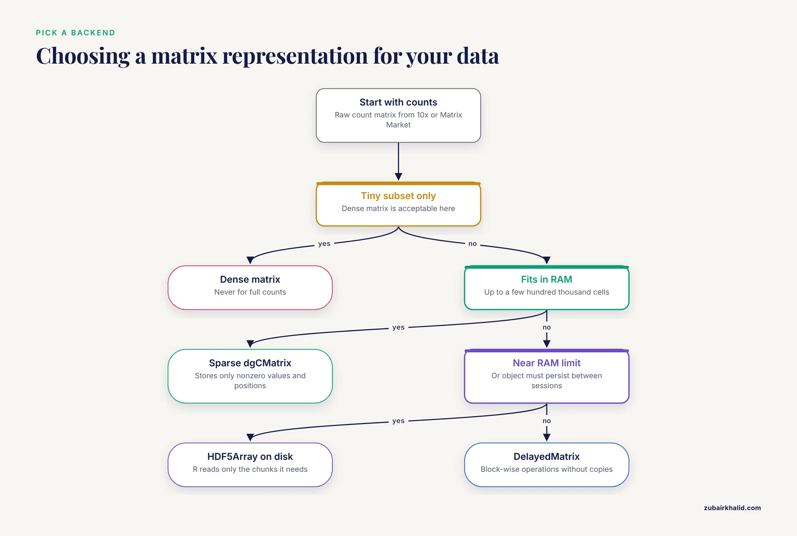
Three representations cover almost every situation you will meet.
- Sparse in-memory matrices (
dgCMatrixfrom theMatrixpackage). The default output of 10x Genomics pipelines and the working format for datasets up to a few hundred thousand cells. - Delayed operations on in-memory or on-disk arrays (
DelayedArray,DelayedMatrix). Wraps a matrix so that operations are recorded and executed block by block instead of materializing full intermediate results. - On-disk backed arrays (
HDF5Array). The matrix lives in an HDF5 file on disk and R reads only the chunks it needs. This is what makes million-cell analyses possible on a laptop.
The table below summarizes when to use each.
| Representation | Key packages | Memory footprint | Use when |
|---|---|---|---|
Dense matrix | base R | Full cells x genes, always | Only for tiny subsets, never for full counts |
Sparse dgCMatrix | Matrix | Proportional to nonzero count | Standard choice for counts up to a few hundred thousand cells |
DelayedMatrix (in memory) | DelayedArray | Same as underlying data, avoids copies | You want block-wise operations without copies |
HDF5Array (on disk) | HDF5Array, DelayedArray | Near zero in RAM for the matrix | Very large datasets, or you need the object to survive between sessions |
SingleCellExperiment with HDF5 assay | SingleCellExperiment, HDF5Array | Matrix on disk, metadata in RAM | Full Bioconductor workflows at scale |
The Bioconductor SingleCellExperiment container holds counts, metadata, and reduced dimensions in one object, and it accepts any of these matrix backends. Almost every Bioconductor single-cell package works with it, which is why it is the backbone of most R for bioinformatics single-cell pipelines.
Step-by-Step: A Memory-Conscious Workflow
The numbered walkthrough below moves a large dataset from raw files to clustered, annotated, analysis-ready form. Code uses a hypothetical experiment of about 1 million cells and 20,000 genes. Substitute your own paths and sizes.
Step 1. Measure Before You Optimize
Run this before changing anything so you know where memory actually goes.
install.packages("pram")        # not needed if already installed
# Count matrix memory in a session that just loaded the data
counts <- readRDS("counts_1M.rds")        # example dense matrix
format(object.size(counts), units = "GB")
#> 160.4 Gb

# Peak memory used by the current R process
pram::ram()      # or use the `gcinfo(TRUE)` toggle for automatic reports
gc()
#>           used    (Mb) gc trigger   (Mb)  limit (Mb)  max used  (Mb)
#> Ncells  512341  27.4     1094323   58.5        NA    784213  41.9
#> Vcells 2.1e+09 16012.7  2.6e+09 19827.5        NA  2.2e+09 16845.5
The Vcells row under used (Mb) approximates your data footprint. If a single load already consumes most of your RAM, later steps will fail with the classic error:
Error: cannot allocate vector of size 156.8 GbThis error means R asked the operating system for a block of memory and did not get it. The fix is almost always a representation change, not more RAM.
Step 2. Load Counts as Sparse Matrices
Never read a count matrix into R as dense text. The 10x format is already sparse, so use a reader that preserves that.
library(SingleCellExperiment)
library(DropletUtils)

sce <- read10xCounts("filtered_feature_bc_matrix/", type = "HDF5Matrix")
sce
#> class: SingleCellExperiment
#> dim: 20000 982458
#> metadata(1): Samples
#> assays(1): counts
#> rownames(20000): ENSG00000243485 ENSG00000237613 ... ENSG00000277475 ENSG00000278633
#> colnames(982458): AAACCCAAGAAACACT-1 AAACCCAAGAAACATG-1 ...
#> colData names(1): Barcode
Key parameters:
type = "HDF5Matrix"keeps the counts on disk inside a sparse HDF5 file rather than RAM. Usetype = "Sparse"for an in-memory sparse matrix if your dataset fits comfortably.- The returned object is a
SingleCellExperimentwith a sparse, delayedcountsassay.
If your data starts as a Matrix Market file or a data frame of triplets, build the sparse matrix directly:
library(Matrix)
counts <- readMM("matrix.mtx")                      # sparse, in memory
# or from a triplet table of gene index, cell index, count
trip <- read.delim("counts_triplets.tsv")
counts <- sparseMatrix(i = trip$gene, j = trip$cell, x = trip$count,
                       dims = c(n_genes, n_cells))
Check that it worked by confirming the class and the sparsity:
class(counts(sce))
#> [3] "HDF5SparseMatrix"
#> attr(,"package")
#> [3] "DelayedArray"
sum(counts(sce) == 0) / length(counts(sce))
#> The result is typically 0.85 to 0.95 for UMI data
That last check is expensive on huge matrices, so run it on a column subset:
sub <- counts(sce)[, 1:5000]
mean(sub == 0)
Step 3. Move Existing Data to Disk with HDF5
If you already have a large sparse matrix in memory and need to free RAM, convert it to an on-disk representation.
library(HDF5Array)
setAutoRealizationBackend("HDF5Array")

sparse_counts <- as(counts, "dgCMatrix")          # if not already sparse
h5_counts <- writeHDF5Array(sparse_counts, "counts.h5", "counts",
                            chunkdim = c(1000, 1000))
sce <- SingleCellExperiment(assays = list(counts = h5_counts))
gc()
Key parameters:
chunkdimcontrols how the file is blocked. Chunks of roughly 1,000 by 1,000 balance row-wise operations (gene statistics) and column-wise operations (cell statistics). A very tall, thin chunk speeds gene-wise ops and slows cell-wise ops.writeHDF5Arrayleaves the original in-memory object untouched, so callrm()on it andgc()afterwards to actually free RAM.
A common failure here is disk exhaustion. HDF5 conversion needs temporary space about the size of the final file. For a 1 million by 20,000 matrix at roughly 10 percent density, expect on the order of 20 to 30 GB on disk, plus temporary space during writing.
Step 4. Choose a Memory-Efficient PCA
PCA is usually the first heavy computation in a scRNA-seq workflow, and benchmarks show that the implementation matters more than most analysts assume. The Tsuyuzaki benchmark evaluated fast and memory-efficient PCA algorithms on large-scale scRNA-seq data and found Krylov-subspace methods and randomized SVD both fast and accurate, with a guideline for choosing among them based on the user's computing environment [2]. In practice this means using iterative partial SVD rather than full SVD.
library(scater)
library(BiocSingular)
library(scran)

sce <- logNormCounts(sce)                       # delayed, block-wise log-normalization
genes_hv <- getTopHVGs(sce, n = 2000)           # restrict to highly variable genes
sce <- runPCA(sce, subset_row = genes_hv, ncomponents = 30,
              BSPARAM = IrlbaParam(), BPPARAM = MulticoreParam(4))
Key parameters:
subset_rowreduces the problem from 20,000 genes to 2,000 highly variable genes. This alone cuts PCA time and memory roughly tenfold and is standard practice.BSPARAM = IrlbaParam()selects the truncated (IRLBA) algorithm, one of the Krylov-subspace approaches found efficient and accurate in the benchmark [2].RandomParam()gives randomized SVD, the other strong family from the same benchmark [2].ncomponents = 30is a common choice for downstream UMAP and clustering. Compute more only if you need them.BPPARAMcontrols parallel workers. Match it to your physical cores.
The result is stored as a small dense matrix inside the object (1 million cells by 30 dimensions is about 240 MB as doubles), which is fine.
If you get Error in svd(X, nu = k, nv = k) : infinite or missing values in 'x', you have NaNs in your normalized matrix, usually from genes with zero total counts. Filter those genes before PCA:
sce <- sce[rowSums(counts(sce)) > 0, ]For even more appropriate modeling of count data, Poisson GLM-PCA offers a count-aware alternative to PCA. The fastglmpca package implements Alternating Poisson Regression, which produces better-quality fits in less time than earlier GLM-PCA algorithms and is memory-efficient and parallelizable, properties that help with large scRNA-seq datasets [4].
library(fastglmpca)
# fit a Poisson GLM-PCA on the count matrix for a subset of genes
fit <- fit_glmpca_poisson(counts(sce)[genes_hv, ], K = 30)
GLM-PCA is slower than ordinary PCA even when accelerated, so use it when count-aware dimension reduction matters for your question, and reserve fast PCA for routine exploratory workflows.
Step 5. Cluster Without Holding Everything in RAM
Standard k-means requires the full data in memory. Two scalable alternatives cover most needs.
Mini-batch k-means with on-disk data. The mbkmeans package implements mini-batch k-means for single-cell data and supports on-disk representations such as HDF5, so the full matrix never needs to be loaded at once. Its developers demonstrated performance on a dataset with 1.3 million cells [5].
library(mbkmeans)
pcs <- reducedDims(sce)$PCA                     # 1M x 30, fits in memory
clust <- mbkmeans(pcs, clusters = 15,
                  batch_size = 500,
                  num_init = 3,
                  max_iters = 100)
sce$mbk <- clust$iters.per.sample
table(clust$Cluster)                            # inspect cluster sizes
Key parameters:
clustersis k, the number of clusters. Unlike standard k-means you must fix it in advance.batch_sizeis the number of cells drawn per mini-batch. Values in the low hundreds to low thousands work well and keep each iteration cheap.num_initis the number of random starts. Three to five guards against poor local optima at modest cost.
Subsample, cluster, then classify. The SSCC framework clusters a representative subsample and then classifies the remaining cells, using random projection and feature construction. On a dataset of 68,578 human blood cells, SSCC improved clustering accuracy by 20 percent and ran about 50 times faster than SC3 while using only 66 percent of the memory, and improved accuracy up to threefold over k-means [3]. The R implementation is available as the sscClust package [3].
# sscClust from https://github.com/Japrin/sscClust
library(sscClust)
# workflow: cluster a subsample, then project labels onto all cells
This subsample-then-classify pattern generalizes beyond SSCC and is one of the most reliable memory tips for very large data: expensive steps run on tens of thousands of cells, cheap prediction steps label the rest.
To choose the number of clusters, treat algorithm estimates as one input rather than ground truth. A systematic benchmark of clustering algorithms on Tabula Muris-derived datasets, including high-cell-number Tabula Muris and Tabula Sapiens data, measured how well methods recover the true number of cell types and compared deviation of the estimate, variability, concordance with known labels, running time, and peak memory [1]. The benchmark's accompanying resource summarizes the strengths and weaknesses of each method so you can match an algorithm to your dataset's cell type composition [1].
Step 6. Scale Differential Expression with Pseudobulk
Cell-level differential expression tests treat cells as independent replicates, which ignores biological replication and scales poorly. The pseudobulk approach aggregates counts per donor and cell type, then fits standard bulk RNA-seq models, which is both statistically sound and computationally cheap. The dreamlet package implements this with precision-weighted linear mixed models and was designed for large cohorts, where it is substantially faster and uses less memory than existing workflows while supporting complex models. It was demonstrated on a dataset of 1.4 million single nuclei from postmortem brains of 150 Alzheimer's disease cases and 149 controls [6].
library(dreamlet)

# pseudobulk per donor and cell type, then mixed model per gene
pb <- aggregateAssays(sce, sample_id = "donor", celltype_id = "celltype")
res <- processAssays(pb, ~ disease + age + sex,
                     min.cells = 10, min.count = 10)
fit <- dreamlet(res, ~ disease + age + sex)
de <- eamp(fit, coef = "diseaseAD")
Key parameters:
min.cellsdrops donor-by-celltype aggregates below a cell count threshold, avoiding noisy pseudobulk profiles.min.countfilters lowly expressed genes before modeling.
The memory win comes from the collapse: 1 million cells become a few hundred donor-by-celltype matrices, and the models run on those.
Step 7. Score Gene Sets Efficiently
Gene set scoring per cell (module scores, signatures) is a common step that analysts implement with slow row-wise loops. The PLAID algorithm performs single-sample gene set enrichment with sparse matrix computation and was built specifically to cut the runtime and memory demands that make existing methods impractical on large-scale single-cell datasets [7]. It integrates several widely used scoring algorithms in one interface [7].
# PLAID: ultrafast single-sample gene set scoring, sparse-matrix based
# see the package documentation for the current function interface
The general principle applies regardless of tool: express per-cell scores as sparse matrix operations, never as apply() loops over genes.
Step 8. Convert Between R and Python Formats Carefully
Mixed R and Python pipelines are common, and the two ecosystems do not share a native format. A systematic benchmark of five conversion tools (Zellkonverter, anndataR, convert2anndata, easySCF, CrossCell) across 68 datasets from 1,438 to 1,665,937 cells found substantial gaps in H5AD-to-RDS conversion, including implicit type changes across the language boundary, such as Int32 counts becoming Float64, that can affect downstream compatibility. Existing tools already failed extensively on datasets below 74,000 cells, and the Rust-based CrossCell toolkit achieved 100 percent success across the standard benchmark datasets with 2.5 to 4.9 times the speed and 37 to 61 percent memory savings over competing tools, converting CELLxGENE datasets up to 1.67 million cells [8].
# Reading an H5AD file into Bioconductor
library(Zellkonverter)
sce <- readH5AD("large_dataset.h5ad", X = "HDF5Array")

# Verify integer counts survived the conversion
storage.mode(counts(sce)[1:100, 1:100])
#> If values print as numeric rather than integer, the type changed in transit
Two habits make conversions safe. First, after any H5AD-to-R conversion, check that the count assay is still integer-typed and that metadata column classes (factors, dates, logicals) match what you wrote. Second, keep a checksum of cell and gene identifiers before and after conversion so silent reordering is caught immediately.
Step 9. Save Smartly
Save the sparse, disk-backed object, not a dense copy.
saveRDS(sce, "analysis_1M.rds")           # metadata + small matrices in RAM-sized file
# The HDF5-backed assay stays in counts.h5 and is referenced by the RDS
For reproducible pipeline checkpoints, also write the reduced dimensions and cluster labels as plain CSVs so collaborators can inspect results without R.
Common Mistakes and Limitations
- Calling
as.matrix()on a sparse matrix. This is the single fastest way to fill RAM. A one-line summary or a small slice does not need densification. UseMatrix::summary()or index a few columns instead. - Row-wise
apply()loops over genes. Each iteration can copy data. Vectorize withrowSums,rowMeans,Matrix::colSums, orDelayedArrayblock operations. On an HDF5-backed matrix, set a sensible block size withsetAutoBlockSize()so each pass streams through the file once. - Storing counts as doubles. UMI counts are small nonnegative integers. A double takes twice the memory of an integer. When building matrices yourself, ensure
xis integer, and after conversions checkstorage.mode(), since cross-language type drift such as Int32 to Float64 has been documented as a real failure mode in format conversion [8]. - Keeping both copies during conversion. Writing an HDF5 copy while the in-memory object still exists doubles peak usage. Convert, then
rm(old_counts)andgc()immediately. - Running PCA on all genes. Full-gene PCA wastes time on noise and memory on zeros. Selecting a few thousand highly variable genes first is standard, and choosing a fast algorithm matters. Krylov-subspace and randomized SVD methods are the efficient and accurate choices on large scRNA-seq data [2].
- Using dense k-means on million-cell matrices. Use mbkmeans, which reads on-disk HDF5 data and was demonstrated at 1.3 million cells [5], or a subsample-and-classify strategy such as SSCC [3].
- Trusting a single estimated cluster number. Estimates of the number of cell types vary between algorithms and with cell type proportion imbalance. The benchmark work behind this point evaluated algorithms across many sampled datasets and reported both deviation and variability of the estimates [1]. Treat the estimate as a hypothesis to check with marker genes.
- Testing cells as independent replicates. For multi-donor studies, pseudobulk aggregation with tools like dreamlet is both the statistically defensible and the memory-feasible route, as demonstrated at the scale of 1.4 million nuclei across 299 subjects [6].
- Ignoring session hygiene. Large objects accumulate. Call
rm()on intermediates, rungc()after big steps, and restart R between major stages. On macOS, if R aborts withvector memory exhausted (limit reached?), raise the limit by launching R with a largerR_MAX_VSIZEenvironment value. - Assuming every analysis scales the same way. Some tasks are inherently heavier. Benchmark evidence from clustering work shows running time and peak memory differ substantially across algorithms on the same data [1], so profile your own pipeline rather than trusting defaults.
One honest limitation of R itself: script-based environments like R can struggle with very large-scale data unless the analysis is built around sparse and disk-backed representations from the start. This constraint motivated memory-aware designs across computational biology, and the packages above exist precisely because naive in-memory code stops working at scale [5]. Plan the data representation before writing analysis code, not after the first crash.
Quick Reference: Memory-Saving Defaults
| Task | Default to avoid | Memory-saving replacement | Package |
|---|---|---|---|
| Reading 10x data | read.csv into dense matrix | read10xCounts(type = "HDF5Matrix") | DropletUtils |
| Normalization | log2(counts + 1) on dense copy | logNormCounts() on delayed assay | scater/scran |
| PCA | Full prcomp() | runPCA(BSPARAM = IrlbaParam()) on HVGs | scater, BiocSingular |
| Count-aware DR | Iterative GLM-PCA | Alternating Poisson Regression | fastglmpca [4] |
| Clustering | kmeans() on full matrix | mbkmeans() on HDF5 or subsample-then-classify | mbkmeans [5], sscClust [3] |
| Differential expression | Per-cell tests | Pseudobulk mixed models | dreamlet [6] |
| Gene set scoring | Per-cell loops | Sparse-matrix scoring | PLAID [7] |
| Session cleanup | Nothing | rm() plus gc() after each big step | base R |
Frequently Asked Questions
How much RAM do I need for 1 million cells?
With an HDF5-backed count matrix and a sparse workflow, 32 to 64 GB is workable for most analyses, because the counts stay on disk and only small matrices like PCA scores and metadata sit in RAM. Dense representations would need on the order of 160 GB for the counts alone.
Should I use Seurat or Bioconductor for large single-cell data?
Both work, but Bioconductor's SingleCellExperiment with DelayedArray and HDF5Array gives you the most direct control over on-disk data, and packages such as mbkmeans and dreamlet are built around it. Many analysts use Seurat for interactive exploration and Bioconductor for large-scale pipelines.
What is the single biggest memory saving in R for scRNA-seq?
Never materialize dense copies of the count matrix. Load counts as sparse, restrict analyses to highly variable genes, and move the matrix to HDF5 when it no longer fits in RAM.
Can I cluster a million cells on a laptop?
Yes, if you pick the right algorithm. Mini-batch k-means with on-disk HDF5 data was demonstrated on 1.3 million cells [5], and subsample-then-classify approaches such as SSCC reduce both memory and runtime while improving accuracy [3].
When should I use HDF5-backed data instead of a sparse in-memory matrix?
Use HDF5 when the sparse matrix approaches your RAM limit, when you want objects to persist between sessions without reloading, or when the package you are using supports on-disk streaming. Stay in memory for datasets that fit comfortably, since in-memory operations are faster.
Why is my PCA slow, and how do I fix it?
You are probably running full SVD on all genes. Restrict to about 2,000 highly variable genes and use a truncated algorithm such as IRLBA or randomized SVD, both of which benchmark as fast, memory-efficient, and accurate on large scRNA-seq data [2].
How do I safely convert between H5AD and RDS?
Use a maintained converter, then verify the result: check that the count assay kept its integer type, that metadata classes survived, and that cell and gene identifiers match the original. Conversion benchmarks document implicit type changes and failures at scale, so verification is not optional [8].
How do I do differential expression across many donors and millions of cells?
Aggregate to pseudobulk per donor and cell type, then fit bulk-style mixed models with dreamlet, which is faster and more memory-efficient than alternative workflows at cohort scale and was validated on 1.4 million nuclei across hundreds of subjects [6].
Sources
- Benchmarking clustering algorithms on estimating the number of cell types from single-cell RNA-sequencing data.
- Benchmarking principal component analysis for large-scale single-cell RNA-sequencing.
- SSCC: A Novel Computational Framework for Rapid and Accurate Clustering Large-scale Single Cell RNA-seq Data.
- Accelerated dimensionality reduction of single-cell RNA sequencing data with fastglmpca.
- mbkmeans: Fast clustering for single cell data using mini-batch k-means.
- Efficient differential expression analysis of large-scale single-cell transcriptomics data using Dreamlet.
- PLAID: ultrafast single-sample gene set enrichment scoring.
- Benchmarking single-cell format conversion tools reveals interoperability gaps and introduces CrossCell for reliable cross-ecosystem data exchange.