Handling Large Genomic DataFrames in Python
By Dr. Zubair Khalid, DVM, MS, PhD ·

The most common cause of memory failure with a large genomic DataFrame in pandas is loading every column with default 64-bit dtypes and storing strings as Python objects. A VCF or BED file that looks modest on disk, say 2 GB of compressed text, can balloon to 20 GB or more in RAM once pandas assigns int64 to positions, float64 to every numeric field, and object arrays to chromosome names, variant IDs, and gene symbols. The first thing to check is not your hardware. It is df.memory_usage(deep=True) on the DataFrame you already loaded, or pd.read_csv(..., nrows=1000).memory_usage(deep=True) on a sample if you have not loaded it yet. That single call tells you which columns eat the memory and whether the problem is dtypes, strings, or row count.
This guide walks through the causes of large genomic DataFrame memory problems in pandas, from the most common to the rarest, gives a diagnostic sequence you can follow in under ten minutes, and lays out the fixes in order of effort. The same principles apply whether you are handling large genomic DataFrames in Python for variant annotation, ChIP-seq peak overlap, or single-cell count matrices.
Why Large Genomic DataFrames Exhaust Memory in pandas
Genomic data has a shape that punishes default pandas behavior. A typical variant table has millions of rows, a dozen columns, and a heavy skew toward categorical text (chromosome, reference allele, alternate allele, consequence terms) mixed with a few large integers (position, end position). Pandas was designed for business tables with thousands of rows, and its defaults reflect that design rather than the shape of genomic intervals.
Pandas has been widely criticized for these inefficiencies and scalability issues, which is exactly the gap that modern engines such as Polars target with a Rust backend built on Apache Arrow [1]. Understanding the specific mechanisms behind the memory blowup is the first step, because each mechanism has a different fix.
Cause 1: Default dtypes carry 64-bit everything
When pandas parses a CSV or TSV, every integer column becomes int64 (8 bytes per value) and every float column becomes float64 (8 bytes per value). A chromosome position never exceeds about 250 million for the human reference genome, which fits comfortably in int32 (4 bytes). Read depth rarely exceeds a few thousand, which fits in int16 or uint16 (2 bytes). A 50 million row DataFrame with four integer columns loaded as int64 spends 1.6 GB on those columns when int32 and int16 would spend 600 MB. Downcasting alone often halves the footprint of a variant table.
Cause 2: Object dtype strings are the hidden tax
This is the mechanism that surprises people most. When pandas stores a column as object, it is not storing the strings in a compact array. It is storing an array of pointers, 8 bytes each on a 64-bit system, plus a full Python string object for every value. A chromosome name like chr1 costs roughly 50 to 60 bytes per row once you count the pointer, the string object header, and the character data. Multiply that by 50 million rows and 6 string columns and you have spent over 15 GB on text that repeats only 25 distinct values. The fix is the category dtype or Arrow-backed strings, covered below.
Cause 3: Loading the whole file when you need a slice
pd.read_csv("variants.vcf", sep="\t", comment="#") reads every field of every record. Most analyses use a fraction of VCF fields. Reading all of FORMAT, all INFO subfields, and all sample genotype columns when your analysis needs only CHROM, POS, REF, ALT, and QUAL multiplies memory by 5 to 20 times for no benefit. The same applies to GTF files, where parsers routinely retain attributes strings that no downstream step reads.
Cause 4: Copies created by operations, not by loading
Even a well-typed DataFrame grows during manipulation. Common sources of hidden copies:
pd.concatin a loop. Each call allocates a fresh DataFrame and copies all prior rows. Appending 1,000 chunks this way does O(n squared) total copying. Collect chunks in a list and concatenate once at the end.df.mergeanddf.joinon keys with duplicates. A many-to-many merge on overlapping positions can turn 10 million rows into 500 million before you see the result. Check key cardinality before merging.groupbyfollowed by aggregation on a poorly typed frame. Group operations build intermediate arrays, and object dtype intermediates multiply the cost.- Chained indexing such as
df[df["chrom"] == "chr1"]["pos"]which can produce copies and triggers the classicSettingWithCopyWarning. df.copy()calls left in code after debugging, andinplace=Truepatterns that do not save memory the way people assume.
Cause 5: The workload is inherently out of core
Some problems are not fixable by typing tricks. A whole-genome intersection of two files with 10 million intervals each produces intermediate results larger than any dtype optimization can rescue on a 32 GB workstation. For interval work specifically, out-of-core and streaming execution is the right answer, and this is precisely the design goal of polars-bio, which implements fast, parallel, and out-of-core operations on large genomic interval datasets using the Apache DataFusion query engine and Apache Arrow for data representation [1].
Troubleshooting Table: Symptom, Cause, Confirmation, Fix
| Symptom | Likely cause | How to confirm | Fix |
|---|---|---|---|
MemoryError during read_csv of a VCF or BED file | Default dtypes plus object strings, whole-file load | Run read_csv with nrows=100000 and compare memory_usage(deep=True) against file size times expected expansion | Specify dtype and usecols at read time, convert strings to category, then load |
| Jupyter kernel dies silently mid-notebook | The OS killed the process, usually during merge, concat, or groupby | Watch RSS with htop or psutil.Process().memory_info().rss while the cell runs | Fix the operation, not the load. Pre-filter rows, verify merge key cardinality, or switch to Polars |
| Memory usage grows with every loop iteration | pd.concat or append inside the loop | Print df.shape and process RSS per iteration, watch quadratic slowdown | Collect chunks in a list, concatenate once after the loop |
| A 2 GB TSV becomes 15 GB in RAM | Object dtype strings and int64 everywhere | df.dtypes shows many object entries, memory_usage(deep=True) dwarfs file size | Convert low-cardinality text to category, downcast numerics, use Arrow-backed dtypes |
df.merge produces far more rows than either input | Many-to-many join on non-unique keys | df["key"].duplicated().sum() on both sides before merging | Aggregate or deduplicate keys first, or join on an interval basis with a genomic library |
CSV loads fine but sort_values or drop_duplicates crashes | Sorting and deduplication allocate full copies | Peak RSS spikes two to three times the frame size during the call | Sort in chunks, or use an engine that streams, or sort on disk with command-line tools |
| Interval overlap on millions of ranges takes hours | Row-wise Python loops or naive pairwise comparison | Profile a 100k row subset, extrapolate | Use an interval library or polars-bio, which ran overlap queries 6.5 times faster than Bioframe on a real-world 10 million versus 1.2 million interval comparison [1] |
| Notebook survives but the machine swaps and freezes | Frame plus operating system cache exceed physical RAM | free -h shows swap in use, htop shows resident memory near capacity | Reduce resident set with chunked processing, or move to out-of-core execution |
| Saved pickle file is enormous and slow to load | Pickle stores object dtype strings verbatim | Compare pickle file size against Parquet export of the same frame | Store in Parquet, which is columnar and compressed, and load with specified dtypes |
A Diagnostic Sequence You Can Follow
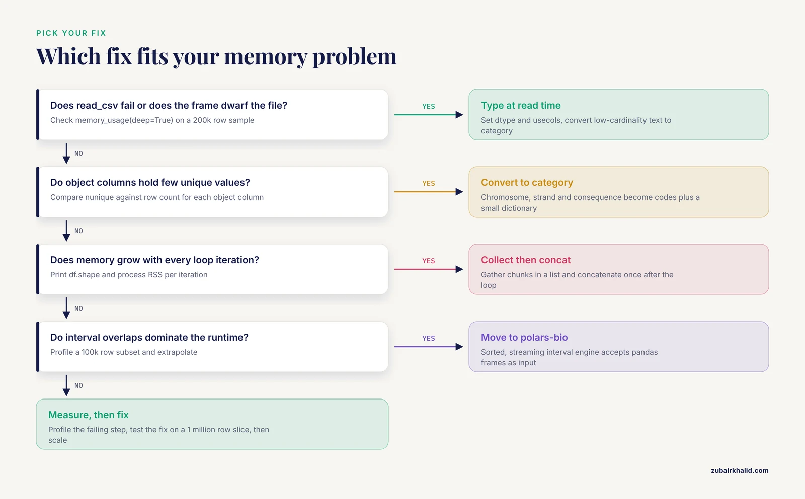
Work through these steps in order. Each one either identifies the cause or eliminates one.
Step 1. Measure before you fix. Run this on a sample:
import pandas as pd

df = pd.read_csv("clinvar_variants.tsv", sep="\t", nrows=200000)
mem = df.memory_usage(deep=True)
print(mem.sort_values(ascending=False))
print(mem.sum() / 1e6, "MB for 200k rows")
deep=True is essential. Without it, pandas reports 8 bytes per object entry and underestimates string memory by roughly an order of magnitude. Extrapolate linearly to your full row count. If the extrapolated number exceeds available RAM, you know the scale of the problem before you commit to a fix.
Step 2. Inspect dtypes and cardinality.
print(df.dtypes)
for col in df.select_dtypes(include="object").columns:
    print(col, df[col].nunique(), "unique of", len(df))
Any object column with fewer than a few thousand unique values across millions of rows is a candidate for category. Chromosome, strand, variant type, consequence class, gene biotype, and filter status all fall in this group.
Step 3. Check the row math. Compare len(df) against what the file should contain. A merge that multiplied rows, or a parser that read sample genotype columns you never intended to use, shows up immediately here.
Step 4. Profile the failing operation, not just the load. If loading succeeds and a later step dies, attach a memory profiler to that step:
from memory_profiler import profile

@profile
def run_overlap():
    # the operation that crashes
    ...

run_overlap()
Alternatively, sample RSS in a background thread or watch htop in a second terminal. The goal is to learn whether the spike happens during parsing, during a copy, or during output materialization.
Step 5. Test the fix on a slice. Never validate a memory fix against the full dataset first. Use a 1 million row subset, verify identical results and a reduced footprint, then scale.
Fix 1: Type the Frame Correctly Before Anything Else
This is the highest return fix for how to fix large genomic DataFrame memory problems, and it costs minutes.
Downcast integers and floats.
ints = df.select_dtypes(include=["int64"]).columns
for c in ints:
    df[c] = pd.to_numeric(df[c], downcast="integer")

floats = df.select_dtypes(include=["float64"]).columns
for c in floats:
    df[c] = pd.to_numeric(df[c], downcast="float")
Position columns become int32, quality scores become float32, and coverage counts become int16 or int32 depending on range. Always check the observed min and max before choosing a downcast, because pandas will not warn you if a value later exceeds the narrower type.
Convert repeated text to category.
cat_cols = ["chrom", "strand", "variant_type", "consequence", "filter_status"]
for c in cat_cols:
    df[c] = df[c].astype("category")
A category column stores each unique string once plus an integer code per row. For a chromosome column with 25 levels across 50 million rows, this replaces roughly 3 GB of Python string objects with about 100 MB of codes plus a tiny dictionary. Category columns also speed up groupby and filtering, because comparisons run on integer codes.
Do the typing at read time, not after. Converting after load means pandas briefly holds the bloated version anyway. Specify dtypes in the reader:
dtypes = {
    "CHROM": "category",
    "POS": "int64",
    "REF": "category",
    "ALT": "category",
    "QUAL": "float32",
    "FILTER": "category",
}
df = pd.read_csv(
    "variants.vcf", sep="\t", comment="#", header=None,
    names=["CHROM", "POS", "ID", "REF", "ALT", "QUAL", "FILTER"],
    usecols=["CHROM", "POS", "REF", "ALT", "QUAL", "FILTER"],
    dtype=dtypes, na_values=".",
)
This pattern alone often turns an unloadable file into a comfortable one. Note that ID was dropped with usecols because variant IDs are high-cardinality strings that resist every optimization.
Consider Arrow-backed dtypes. Recent pandas versions support PyArrow-backed strings and nullable dtypes through dtype_backend="pyarrow" in read_csv or via convert_dtypes(dtype_backend="pyarrow"). Arrow strings store character data contiguously with offsets rather than one Python object per value, which cuts string memory substantially and speeds up string operations. Verify your full dependency stack supports Arrow-backed columns before adopting them in production pipelines.
Fix 2: Load Less, and Load in Chunks
Select columns explicitly. Every usecols argument is memory you never allocate. For a VCF reduced to a BED-like core of chromosome, position, reference, and alternate alleles, this is the difference between loading 30 columns and loading 4.
Read in chunks and process independently. When each chunk can be filtered or aggregated on its own, chunked reading caps peak memory:
chunks = []
for chunk in pd.read_csv("peaks.bed.gz", sep="\t", header=None,
                         names=["chrom", "start", "end", "score"],
                         dtype={"chrom": "category", "start": "int64",
                                "end": "int64", "score": "float32"},
                         chunksize=5_000_000):
    chunks.append(chunk[chunk["score"] > 50])

df = pd.concat(chunks, ignore_index=True)
del chunks
The filtering step shrinks each chunk before concatenation, so the final frame holds only the rows you need. If the analysis is a per-chromosome aggregation, you can aggregate inside the loop and never hold the full frame at all.
Strip headers and metadata at the shell, not in pandas. VCF headers, GTF comment lines, and BED track lines are cheaper to skip with comment="#" or a pre-filtered intermediate than to parse into pandas and drop. Writing a cleaned intermediate file with grep -v "^#" or awk costs seconds and makes every downstream Python load lighter.
Know your file format limits. Plain pandas readers do not parse VCF genotype fields, INFO structured fields, or BCF. For those, a dedicated parser that emits only the fields you need is more memory efficient than any amount of pandas tuning. This is also where the Biopython ecosystem and the wider Python for bioinformatics toolset matter. Biopython's SeqIO and Bio.GenBank parsers stream records as objects rather than materializing everything as one table, which is the right model for sequence-centric work. A practical biopython tutorial point worth internalizing early is that Biopython is built for parsing and sequence manipulation, not for tabular analytics. The efficient pattern is to use Biopython to extract the fields you need into a small typed DataFrame, and leave bulk tabular work to pandas, Polars, or a command-line tool.
Fix 3: Eliminate Hidden Copies and Growth
Concatenate once, outside the loop. This is the single most common performance bug in genomic pandas scripts:
# Wrong: quadratic copying
result = pd.DataFrame()
for path in files:
    result = pd.concat([result, parse_one(path)])

# Right: linear
parts = [parse_one(p) for p in files]
result = pd.concat(parts, ignore_index=True)
Guard merges against cardinality surprises. Before any merge, run left["key"].duplicated().sum() and the same on the right. Genomic coordinates are especially dangerous as merge keys because the same position legitimately appears in many annotations. A many-to-many merge on position can multiply row counts without any error message. For interval-to-interval joins, do not use merge at all. Use an interval-aware library, discussed below, which uses sorted and indexed structures instead of pairwise comparison.
Delete intermediates explicitly. In long notebooks, del big_intermediate combined with gc.collect() after a merge or pivot keeps peak memory bounded. Python does not return memory to the operating system immediately, so a notebook that once held a 10 GB intermediate can report high RSS long after the variable is gone. Restarting the kernel and rerunning only the necessary cells is often the fastest memory fix available.
Avoid chained indexing. Write df.loc[mask, "col"] = value instead of df[mask]["col"] = value. Chained indexing can silently create copies, produce incorrect writes, and trigger SettingWithCopyWarning.
Sort with the index in mind. sort_values allocates a full copy. If you need a sorted frame for interval operations, sort once after loading and persist the sorted result to Parquet so later sessions never pay the cost again.
Fix 4: Persist to Columnar Formats and Memory-Map
Round-tripping genomic tables through CSV wastes both memory and time on every run. Convert cleaned intermediates to Parquet:
df.to_parquet("variants_typed.parquet", index=False)
df2 = pd.read_parquet("variants_typed.parquet")
Parquet stores data columnar and compressed, preserves dtypes including categories, and loads far faster than CSV because pandas skips parsing. A second benefit is selective column loading. pd.read_parquet(path, columns=["chrom", "pos", "ref", "alt"]) reads only those columns from disk, which is the disk-level equivalent of usecols.
For numeric arrays that fit together, NumPy memory mapping with np.load(mmap_mode="r") or np.memmap lets you index into a matrix on disk without loading it, which works well for dense per-position tracks such as coverage arrays.
Fix 5: Move Interval Work to Purpose-Built, Out-of-Core Engines
Interval operations, overlap, nearest neighbor, coverage, and count overlaps, are the core of genomic DataFrame work, and they are exactly where generic pandas behavior fails. Naive implementations compare every interval against every other, which is quadratic. Sorted, indexed algorithms do this in near-linear time, and streaming engines do it without holding both datasets fully in memory.
polars-bio is a Python library built for this problem. Its core is implemented in Rust using the Apache DataFusion query engine and Apache Arrow, and it is compatible with both Polars and pandas DataFrame formats [1]. In a real-world benchmark comparing 10 million query intervals against 1.2 million reference intervals, it ran overlap queries 6.5 times faster, nearest queries 15.5 times faster, count_overlaps 38 times faster, and coverage queries 15 times faster than Bioframe [1]. On equally sized synthetic sets of 10 million against 10 million intervals, the corresponding speedups were 1.6, 5.5, 6, and 6 times [1]. For memory, its streaming mode used 90 times less memory on real interval pairs and 15 times less on synthetic ones in the same evaluation [1].
The practical takeaway is not a specific speedup number but an architectural rule. When your problem is interval algebra on millions of ranges, a specialized engine with sorted data structures and streaming execution outperforms a general-purpose in-memory DataFrame library on both speed and memory. Because polars-bio accepts pandas DataFrames as input, you can keep your existing loading code and replace only the overlap step [1].
Polars itself is worth adopting for the non-interval parts of the same pipelines. Its Rust backend and lazy execution mean the query optimizer can push filters down and stream results rather than materializing full intermediates, which addresses the scalability criticisms aimed at pandas [1]. A typical migration for a genomic pipeline looks like this:
import polars as pl

lf = (
    pl.scan_csv("variants.tsv", separator="\t", comment_prefix="#")
      .select(["CHROM", "POS", "REF", "ALT", "QUAL"])
      .filter(pl.col("QUAL") > 30)
      .group_by("CHROM")
      .len()
)
result = lf.collect()  # or .collect(engine="streaming") for out-of-core
scan_csv builds a lazy plan without reading the file. Filters are applied during scan, and only the reduced result materializes. For files larger than RAM, streaming collection keeps peak memory bounded.
Fix 6: Use the Right Tool at the Right Stage
Not every step of a genomic workflow belongs in a DataFrame. Mature pipelines distribute work:
- Streaming text tools such as
bgzip,tabix,awk, andsorthandle per-line filtering and sorting of BED and VCF-scale files with constant memory, and they parallelize trivially. Pre-filtering a 40 GB VCF down to the 2 GB relevant to one chromosome before Python ever sees it is the cheapest memory fix that exists. - Command-line interval tools perform whole-genome intersections and merges in bounded memory with sorted input.
- Databases such as SQLite, DuckDB, or a managed warehouse hold tables larger than RAM and answer filtered queries without any Python memory pressure. DuckDB in particular queries Parquet files directly with an API that feels like pandas.
- Biopython handles sequence records, annotations, and format conversion where record-at-a-time streaming fits, complementing rather than replacing DataFrame tools.
The general pattern for handling large genomic DataFrames in Python at scale is to shrink the data as early in the pipeline as possible, keep it in typed columnar formats from then on, and reserve full in-memory pandas for the small, final analytical tables.
Worked Example: A 30 GB VCF Annotation Task on a 32 GB Machine
Consider a concrete case. You have a joint-called VCF with 800 million variant records across 2,000 samples and need a per-gene count of high-impact variants. Loading the full VCF into pandas is impossible. A working sequence:
- Extract one chromosome at a time with
bcftools viewortabix, writing stripped TSVs containing only CHROM, POS, GENE, and consequence. - Read each chromosome TSV with the
dtypedictionary shown earlier, filter to high impact, and aggregate to a per-gene count in the loop. - Collect the 25 small per-chromosome aggregate frames, concatenate once, and write the result to Parquet.
Peak memory never exceeds the size of one chromosome's typed frame, roughly 1 to 2 GB, and total runtime is dominated by the shell-level extraction. This is the chunk-and-aggregate pattern in Fix 2 combined with early filtering from Fix 6, and it scales to far larger files than the machine could ever hold in RAM.
Prevention Practices
- Type every read. Never call
read_csvwithoutdtypeandusecolsin a production pipeline. Write a sharedload_variants()helper so typing rules live in one place. - Assert memory budgets. After every load, assert
df.memory_usage(deep=True).sum() < BUDGET. A failing assertion in CI catches dtype regressions before they crash a 12-hour pipeline at hour 10. - Persist typed intermediates. Once a table is filtered and typed, write Parquet. Downstream steps read Parquet and inherit correct dtypes for free.
- Ban concat-in-loops in code review. It is easy to write, invisible in tests on small data, and quadratic in production.
- Benchmark interval operations on realistic sizes. Synthetic 1,000-row tests hide the memory behavior that appears at 10 million rows. Run timing and RSS checks on at least one real-scale file.
- Log peak RSS, not just runtime. A step that runs in 40 seconds but spikes to 90 GB is more dangerous than one that runs in 4 minutes with flat memory. Tools like
/usr/bin/time -vreport maximum resident set size for any command.
Common Mistakes and Limitations
- Trusting
df.info()for memory decisions. Withoutmemory_usage="deep",inforeports 8 bytes for every object entry and understates string memory by roughly an order of magnitude. Always usedeep=Truefor object columns. - Downcasting without range checks.
downcast="integer"is safe on load because pandas inspects actual values, but manually assigningint16to a column that later receives a larger value silently overflows. Check min and max, and prefer unsigned types for counts. - Category dtype is not always a win. Columns with high cardinality, such as variant IDs, free text, or full sequences, grow when converted to category because the dictionary plus codes exceeds the original storage. Convert only columns with genuinely few unique values, and verify with
memory_usage(deep=True)before and after. - Assuming
inplace=Truesaves memory. Most pandasinplaceoperations still allocate the result internally. The parameter avoids one binding, not the allocation. - Forgetting that the kernel remembers. In Jupyter, deleting a variable does not guarantee the memory returns promptly to the OS. Restarting the kernel and rerunning from Parquet checkpoints is the reliable reset.
- Interval joins via merge. Position-based many-to-many merges are a row explosion waiting to happen. Interval libraries exist for this reason.
- One fix rarely suffices at scale. Dtype optimization handles the 5 to 20 GB case. The 100 GB case requires streaming, out-of-core execution, or a database. Match the fix to the scale.
- Individual analyses vary. Memory behavior depends on your specific columns, dtypes, and operations. Profile your own pipeline rather than borrowing numbers from someone else's benchmark, including the ones in this article.
Frequently Asked Questions
Why does my 2 GB VCF use 20 GB of RAM in pandas?
Pandas assigns int64 and float64 to every numeric column and stores text as Python object arrays, which cost roughly 50 to 60 bytes per value including pointers and object headers. VCF files also contain far more columns than most analyses need. Specifying dtype, usecols, and category conversion at read time typically cuts this by 5 to 10 times.
How do I check how much memory a pandas DataFrame actually uses?
Run df.memory_usage(deep=True) and sum the result. The deep=True argument forces pandas to measure real string sizes instead of assuming 8 bytes per object entry. Compare the total against your available RAM, and look at the per-column breakdown to find the worst offenders.
What is the fastest way to reduce DataFrame memory before trying anything else?
Convert low-cardinality string columns to category, downcast integers with pd.to_numeric(..., downcast="integer"), downcast floats to float32, and reload with usecols to drop columns you never use. These four steps take minutes and often cut memory by half or more.
When should I stop optimizing pandas and switch to Polars?
Switch when a single DataFrame exceeds roughly a quarter of your RAM, when you concat in loops, or when interval operations dominate runtime. Polars uses a Rust backend with lazy, streamable execution that avoids materializing full intermediates, and polars-bio adds parallel, out-of-core genomic interval operations compatible with both Polars and pandas inputs.
Can pandas handle data larger than RAM at all?
Only through chunked processing with chunksize in read_csv, and only when each chunk can be filtered, aggregated, or written independently. Chunking does not help operations that require the full table at once, such as a global sort or a whole-genome join. Those need an out-of-core engine or a database.
Do I need Biopython for large genomic tables?
Biopython is the right tool for sequence records, GenBank and FASTA parsing, and format conversion, where streaming record-by-record keeps memory flat. For large tabular genomic data such as VCF, BED, and GTF, pandas, Polars, or command-line tools are usually better suited. The efficient pattern is Biopython to extract fields into a small typed table, then a DataFrame engine for bulk analysis.
Why does my DataFrame get bigger after a merge?
Merges on keys that appear more than once in either table produce every combination of matching rows. A many-to-many merge on genomic position, where the same position legitimately maps to many annotations, can multiply millions of rows into hundreds of millions. Check duplicated().sum() on both merge keys first, and use an interval-aware library for coordinate joins.
What memory figure should I plan for when loading a genomic CSV?
Measure it rather than guessing. Load 100,000 rows with nrows, call memory_usage(deep=True), sum it, and extrapolate by row count. As a rough prior, typed genomic tables with category columns land near 2 to 5 times compressed file size, while default-typed loads with object strings commonly reach 10 to 20 times. Your measured number from a real sample beats any rule of thumb.