How to Use IRanges for Genomic Interval Arithmetic in R
By Dr. Zubair Khalid, DVM, MS, PhD ·

By the end of this iranges tutorial on genomic intervals, you will be able to build interval objects in R, shift and resize them, merge overlapping ranges, run overlap queries between two sets of intervals, compute per-base coverage, and check your own work for the off-by-one errors that cause most interval bugs. The article is a step-by-step bioconductor tutorial aimed at people doing r for bioinformatics work who have basic R skills but no prior Bioconductor experience.
What you need on hand:
- R 4.x installed (any recent version works)
- The BiocManager package, which you will use to install IRanges
- About 30 minutes
Why Genomic Interval Arithmetic Matters
Almost every next-generation sequencing workflow reduces to the same core problem at some point: you have intervals on the genome (peaks, variants, reads, exons) and you need to ask how they relate to other intervals (promoters, gene bodies, known binding sites). NGS experiments routinely produce genomic loci that represent genetic variation, transcription factor occupancy, or histone modifications, and interpreting those loci requires comparing them against known genomic and epigenomic annotations [1]. That comparison is interval arithmetic: overlaps, unions, intersections, distances, and coverage.
IRanges is the Bioconductor package that implements these operations on plain integer ranges. It is the foundation underneath GenomicRanges, which adds chromosome names and strand. Even if you end up working mostly with GRanges, you need to understand IRanges, because every GenomicRanges call delegates the actual interval math to it. Higher-level annotation and enrichment tools, including GLANET, sit on this same conceptual layer: they take user-supplied loci, intersect them with a library of gene sets and genomic features, and run statistical enrichment tests [1].
Installing and Loading IRanges
IRanges is a core Bioconductor package. Install it through BiocManager:
if (!requireNamespace("BiocManager", quietly = TRUE))
    install.packages("BiocManager")

BiocManager::install(c("IRanges", "GenomicRanges"))
Then load it and confirm the version:
library(IRanges)
packageVersion("IRanges")
Expected output looks like this (your version may differ):
[1] '2.32.0'If installation fails, the usual cause is an out-of-date R version. Bioconductor releases are tied to specific R versions, so update R first, then retry.
Step-by-Step IRanges Tutorial for Genomic Intervals
The walkthrough below uses three toy intervals that behave like ChIP-seq peaks on one chromosome. The numbers are small so you can verify every result by hand.
Step 1: Create an IRanges Object
An IRanges object stores a start, an end, and a width for each interval. The invariant is always width = end - start + 1 because coordinates are 1-based and closed on both ends, meaning the start and end positions themselves are included.
ir <- IRanges(start = c(10, 12, 18), end = c(15, 20, 25))
ir
Expected output:
IRanges object with 3 ranges and 0 metadata columns:
          start       end     width
      <integer> <integer> <integer>
  [1]        10        15         6
          12        20         9
          18        25         8
You can also construct a range from a start and a width, which is convenient when a file gives you a length instead of an end coordinate:
IRanges(start = 10, width = 6) # same as 10-15Name your ranges if you plan to merge or split them later, because names survive most operations and let you trace results back to inputs:
names(ir) <- c("peak1", "peak2", "peak3")Step 2: Inspect the Object with Accessors
start(ir)     # 10 12 18
end(ir)       # 15 20 25
width(ir)     #  6  9  8
length(ir)    #  3
sum(width(ir))  # 23, total bases counting overlaps twice
Note the difference between sum(width(ir)) and the width of the merged region. These three peaks span positions 10 through 25 with no gaps between them once merged, so the union covers 16 bases, not 23. Keeping both numbers in mind is one of the most useful iranges tutorial genomic intervals tips: total interval width and nonredundant coverage are different quantities.
Step 3: Resize, Shift, Flank, and Narrow
These four functions are the bread and butter of interval arithmetic. Each returns a new IRanges object and never modifies the input.
resize changes every range to a fixed width, anchored by the fix argument:
resize(IRanges(10, 15), width = 20, fix = "start")IRanges object with 1 range and 0 metadata columns:
start end width
<integer> <integer> <integer>
[1] 10 29 20With fix = "end", the range grows leftward and the start becomes negative if needed. With fix = "center", the range grows evenly in both directions. A common use is trimming peak summits to a fixed window, for example resize(peaks, width = 501, fix = "center") for a 501 bp window centered on each summit.
shift moves every range by a constant:
shift(IRanges(10, 15), 100) # start 110, end 115flank returns the range immediately adjacent to one side:
flank(IRanges(10, 15), width = 3)                  # 7-9, upstream by default
flank(IRanges(10, 15), width = 3, start = FALSE)   # 16-18, downstream
This is how you build promoter windows from transcription start sites: treat each TSS as a one-base range and flank it by 2000 bases upstream.
narrow subsets each range using coordinates relative to the range itself, not the chromosome:
narrow(IRanges(10, 25), start = 6, end = 10) # positions 15-19The sixth base of a range starting at 10 is position 15 on the chromosome. This relative-coordinate behavior surprises people constantly and is covered again in the mistakes section.
Step 4: Merge Overlaps with reduce, disjoin, and gaps
reduce merges overlapping or adjacent ranges into a disjoint, nonredundant set:
ir <- IRanges(start = c(10, 12, 18), end = c(15, 20, 25))
reduce(ir)
IRanges object with 1 range and 0 metadata columns:
start end width
<integer> <integer> <integer>
[1] 10 25 16disjoin cuts the ranges at every start and end boundary so the output ranges never overlap:
disjoin(ir)IRanges object with 5 ranges and 0 metadata columns:
start end width
<integer> <integer> <integer>
[1] 10 11 2
12 15 4
16 17 2
18 20 3
21 25 5gaps returns the uncovered space. For a bare IRanges object the universe is positions 1 through the maximum end, so gaps include the leading region:
gaps(IRanges(start = c(10, 20), end = c(15, 25)))IRanges object with 2 ranges and 0 metadata columns:
start end width
<integer> <integer> <integer>
[1] 1 9 9
16 19 4When you move to GRanges, you can supply seqlengths so gaps and related functions know the full chromosome length and can report the regions beyond the last range as well.
Step 5: Set Operations Between Two Sets of Ranges
The functions union, intersect, and setdiff treat each IRanges object as a set of positions and operate on the merged representation:
x <- IRanges(10, 20)
y <- IRanges(15, 25)

union(x, y)       # one range: 10-25, width 16
intersect(x, y)   # one range: 15-20, width 6
setdiff(x, y)     # one range: 10-14, width 5
If a set operation produces nothing, the result is a zero-length IRanges object rather than an error, so always check length() on results you plan to feed downstream.
Step 6: Find Overlaps Between Two Interval Sets
Overlap queries are the operation you will run most often. The key functions are findOverlaps, countOverlaps, and subsetByOverlaps.
query   <- IRanges(start = c( 5, 12, 30), end = c(10, 18, 35))
subject <- IRanges(start = c( 8, 15, 32), end = c(12, 17, 40))

hits <- findOverlaps(query, subject)
hits
Expected output:
Hits object with 4 hits and 0 metadata columns:
      queryHits subjectHits
       <integer>   <integer>
  [1]         1           1
           2           1
           2           2
           3           3
Each row is one query-subject pair that overlaps. The result is a Hits object, not a data frame, so extract the indices with accessors:
queryHits(hits)    # 1 2 2 3
subjectHits(hits)  # 1 1 2 3
To pull the matching pairs into a data frame for inspection:
data.frame(
  query   = as.character(query[queryHits(hits)]),
  subject = as.character(subject[subjectHits(hits)])
)
countOverlaps answers the per-query version of the same question:
countOverlaps(query, subject)
# [1] 1 2 1
subsetByOverlaps filters the query down to ranges that hit the subject:
subsetByOverlaps(query, subject)
# keeps ranges 12-18 and 30-35
Two parameters control the definition of an overlap:
type:"any"(default, any overlap),"start"(start positions match),"end","within"(query fully inside subject), or"equal".minoverlap: the minimum number of overlapping bases required. The default of 0 means any single-base overlap counts, because a one-base overlap has a width of 1, which passes a minimum of 0. To require at least 10 shared bases, setminoverlap = 10.
findOverlaps(query, subject, minoverlap = 2)Rechecking the pairs by hand, the query range 12-18 overlaps the subject range 8-12 by exactly one base, so that hit disappears when minoverlap = 2 is set and only 3 hits remain.
Step 7: Compute Coverage
coverage converts a set of ranges into a run-length encoded vector reporting how many ranges cover each position:
cov <- coverage(ir)
cov
Expected output:
integer-Rle of length 25 with 6 runs
  Lengths:  9 2 4 2 3 5
  Values :  0 1 2 1 2 1
Reading this: positions 1 through 9 are uncovered, positions 10 and 11 are covered once, positions 12 through 15 are covered by two ranges, and so on. Run-length encoding keeps memory low even for genome-scale data.
Useful checks and summaries:
max(cov)          # 2, the deepest stacking
sum(cov)          # 23, equals sum(width(ir))
mean(cov > 0)     # fraction of 1-25 covered by at least one range: 16/25 = 0.64
The identity sum(coverage(x)) == sum(width(x)) is a fast sanity check that your ranges were constructed correctly.
Step 8: Distance and Nearest-Neighbor Queries
When ranges do not overlap, you often want the gap size or the nearest neighbor:
query   <- IRanges(5, 10)
subject <- IRanges(start = c(30, 90), end = c(40, 95))

nearest(query, subject)     # 1, the first subject is closest
distance(query, subject)    # 19 bases between 10 and 30
distance returns 0 for overlapping ranges, the number of bases strictly between them otherwise. distanceToNearest returns a Hits object with a distance column, and precede and follow return the nearest upstream or downstream subject regardless of distance. These functions drive tasks like assigning peaks to the closest gene.
Step 9: Graduate to GRanges for Real Genomic Data
A bare IRanges object has no chromosome names and no strand. Two ranges on different chromosomes will still be reported as overlapping by findOverlaps, which is almost never what you want in real data. The moment your intervals come from an actual genome, wrap them:
library(GenomicRanges)

gr <- GRanges(
  seqnames = rep("chr1", 3),
  ranges   = ir,
  strand   = "+"
)
gr
GRanges object with 3 ranges and 0 metadata columns:
seqnames ranges strand
<Rle> <IRanges> <Rle>
1 chr1 10-15 +
2 chr1 12-20 +
3 chr1 18-25 +
-------
seqinfo: 1 sequence from an unspecified genomeAll of the IRanges operations above work identically on GRanges, with findOverlaps additionally respecting chromosome and, when ignore.strand = FALSE, strand.
Loading intervals from a BED file is the most frequent real-world conversion, and it is where the classic off-by-one error lives. BED coordinates are 0-based and half-open, meaning the start is excluded conceptually and the end is excluded. Bioconductor coordinates are 1-based and closed. The conversion is:
bed <- data.frame(
  chrom = c("chr1", "chr1"),
  start = c(9999L, 19999L),
  end   = c(10200L, 20400L)
)

gr_from_bed <- GRanges(
  bed$chrom,
  IRanges(start = bed$start + 1L, end = bed$end)
)
A BED record with start 9999 and end 10200 covers chromosome positions 10000 through 10200 inclusive, which is an IRanges of start = 10000, end = 10200, width = 201. GFF and VCF coordinates are already 1-based inclusive, so those formats need no shift.
Quick Reference Table
| Goal | Function | Key arguments | Common pitfall |
|---|---|---|---|
| Build ranges | IRanges(start, end) or IRanges(start, width) | start, end/width | width = end - start + 1, not end - start |
| Merge overlaps | reduce(x) | none | silently reorders and merges |
| Split at boundaries | disjoin(x) | none | output can be longer than input |
| Uncovered space | gaps(x) | none | on bare IRanges the universe starts at 1 |
| Set algebra | union, intersect, setdiff | two IRanges | whole-set operation, not element-wise |
| Element-wise algebra | punion, pintersect, psetdiff | two IRanges of equal length | non-overlapping pairs give zero-width results |
| Overlap query | findOverlaps(query, subject) | type, minoverlap | default counts any 1 bp overlap |
| Per-query counts | countOverlaps(query, subject) | type, minoverlap | returns a vector aligned to query |
| Filter query | subsetByOverlaps(query, subject) | type, minoverlap | input order preserved |
| Fixed-width windows | resize(x, width, fix) | fix = start, end, center | center anchors can go negative |
| Upstream or downstream | flank(x, width, start) | start = TRUE or FALSE | relative to strand in GRanges |
| Relative subsetting | narrow(x, start, end) | start, end | coordinates are relative to each range |
| Per-base depth | coverage(x) | none | returns an Rle, not a vector |
| Nearest neighbor | nearest(x, subject) | none | overlapping ranges have distance 0 |
How to Verify Your Results
Interval code fails quietly, so build checks into every workflow:
- Confirm the invariant on construction:
identical(width(ir), end(ir) - start(ir) + 1L)returns TRUE. - After a merge, confirm the output is nonredundant:
isDisjoint(reduce(ir))returns TRUE. - Confirm coverage arithmetic:
sum(coverage(ir)) == sum(width(ir))returns TRUE. - For a small subset, verify overlaps by hand on paper. Every overlap bug we discuss below is visible in a ten-range example.
- When importing files, compare
sum(width(gr_from_bed))against a column of computed lengths in the source file, such as the width column in a BEDTools summary or a UCSC table export.
Common Mistakes and Limitations
These are the errors that account for the vast majority of wrong results in interval work, along with the exact failure mode each one produces.
1. The BED off-by-one shift. Treating BED start as 1-based produces ranges shifted one base upstream and one base too long. The symptom is subtle: overlaps look roughly correct but boundaries are consistently off, and single-base exonic variants fall just outside your ranges. Fix it once at import with IRanges(bed$start + 1L, bed$end) and never think about it again.
2. Confusing whole-set and element-wise operations. intersect(x, y) merges both inputs first and intersects the merged positions. pintersect(x, y) intersects each pair element-by-element and requires equal lengths. Calling intersect when you meant pintersect returns a plausible-looking object with the wrong number of ranges, and the error often surfaces much later. The same distinction applies to union versus punion and setdiff versus psetdiff. With pintersect, pairs that do not overlap produce zero-width ranges unless you configure the resolve.empty argument, so filter on width(result) > 0 when empties are not meaningful.
3. Using bare IRanges for genome data. If your objects carry no seqnames, findOverlaps will happily report a chr1 peak overlapping a chr9 gene. Always convert to GRanges before overlap queries on real data. This is the single most consequential item on this list.
4. Misreading minoverlap. minoverlap = 0, the default, does not mean zero-overlap hits are returned. It means the minimum requirement is zero, and any range with at least one shared base passes. Setting minoverlap = 1 changes almost nothing. To require meaningful overlap, set the actual base threshold you want.
5. Forgetting that narrow and resize use relative coordinates. narrow(x, start = 1) means the first base of each range, not chromosome position 1. If you write narrow(x, start = 1000) expecting chromosome coordinates, you silently get different windows than intended, or empty ranges for short inputs.
6. Passing non-integer coordinates. Interval starts and ends must be integers. Data read from CSV often arrives as doubles. Construct with IRanges(start = as.integer(df$start), end = as.integer(df$end)). If fractional values sneak in, Bioconductor raises a validity error rather than rounding, typically phrased as a requirement that the values be integer, so fix the source rather than coercing blindly.
7. Expecting an error for invalid ranges and getting one in an unfamiliar place. An end below the start raises a validity error at construction, in the form invalid class "IRanges" object: the end values must be >= start - 1. Note the start - 1, not start: a zero-width range with end = start - 1 is legal and represents an insertion point, which is legal but rarely what you meant when parsing a malformed file. Check for zero widths with width(ir) == 0 after import.
8. Losing track of input identity through reduce. After reduce, individual input peaks that merged together are gone, and the output order is by position, not input order. If you need provenance, name your inputs before merging, or compute overlaps against the original object rather than the reduced one.
9. Treating Hits objects like data frames. hits returns the first hit pair, not the first row of a table. Extract indices with queryHits(hits) and subjectHits(hits) before joining back to metadata.
10. Ignoring strand when it matters. For genomic data, strand-aware overlap of a plus-strand feature against a minus-strand feature is usually wrong unless you explicitly pass ignore.strand = TRUE. The default in GenomicRanges is strand-aware, which surprises people who learned overlap logic from IRanges.
Two honest limitations of IRanges itself. First, it is deliberately context-free: it knows nothing about chromosomes, genomes, strands, or sequence content, so any workflow needing those must move up to GenomicRanges or higher packages. Second, interval arithmetic tells you where features lie, not what they mean biologically. Annotation and enrichment layers add that interpretation. For example, GLANET annotates supplied loci against a library of gene sets and genomic features and performs sampling-based enrichment testing that accounts for GC content and mappability biases, features that raw interval operations cannot model on their own [1]. That statistical layer, and the assessment of its power and Type-I error behavior, is exactly the part IRanges does not provide [1].
Frequently Asked Questions
What is the difference between IRanges and GRanges?
IRanges stores pure integer intervals with no biological context, while GRanges, built on IRanges, adds chromosome names, strand, genome metadata, and per-range annotation columns. Use IRanges for pure arithmetic and GRanges for anything tied to an actual genome.
Are IRanges 1-based or 0-based?
IRanges uses 1-based, fully closed coordinates, so a range from 10 to 15 includes both endpoints and has width 6. BED files use 0-based half-open coordinates, which is why BED imports require adding 1 to every start.
How do I convert a BED file to IRanges?
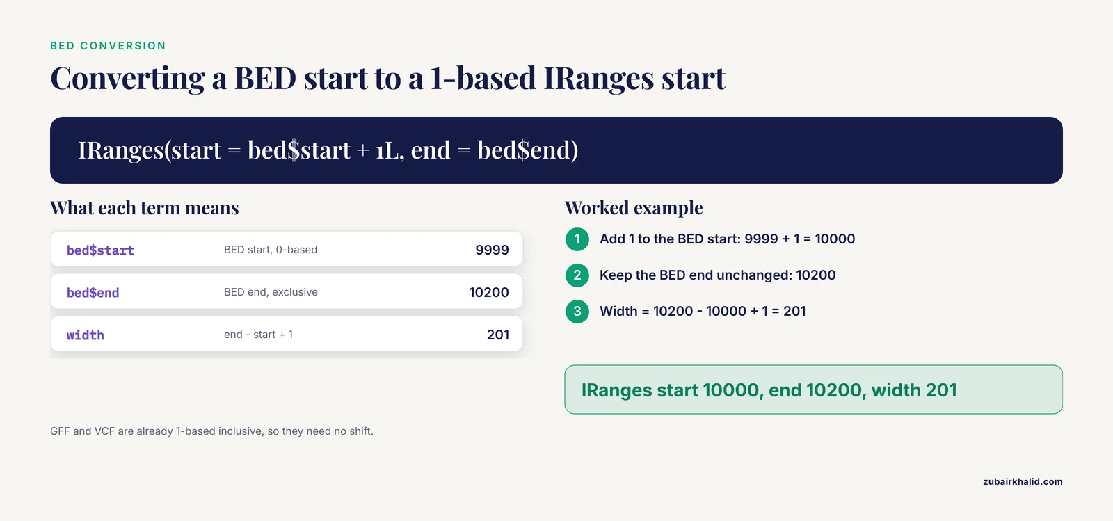
Read the BED file with read.table or rtracklayer::import, then build ranges with IRanges(start = bed$start + 1L, end = bed$end). The end coordinate needs no shift because BED ends are exclusive and Bioconductor ends are inclusive.
What does the reduce function do in IRanges?
reduce merges overlapping and directly adjacent ranges into a sorted, nonoverlapping set. Three peaks at 10-15, 12-20, and 18-25 reduce to the single range 10-25, and the union width drops from 23 to 16 bases.
How do I find which peaks overlap which genes?
Put peaks in one GRanges and genes in another, then call findOverlaps(peaks, genes) and extract index pairs with queryHits and subjectHits. Use type = "within" if you only want peaks fully contained in a gene body.
Why does findOverlaps return zero hits for my data?
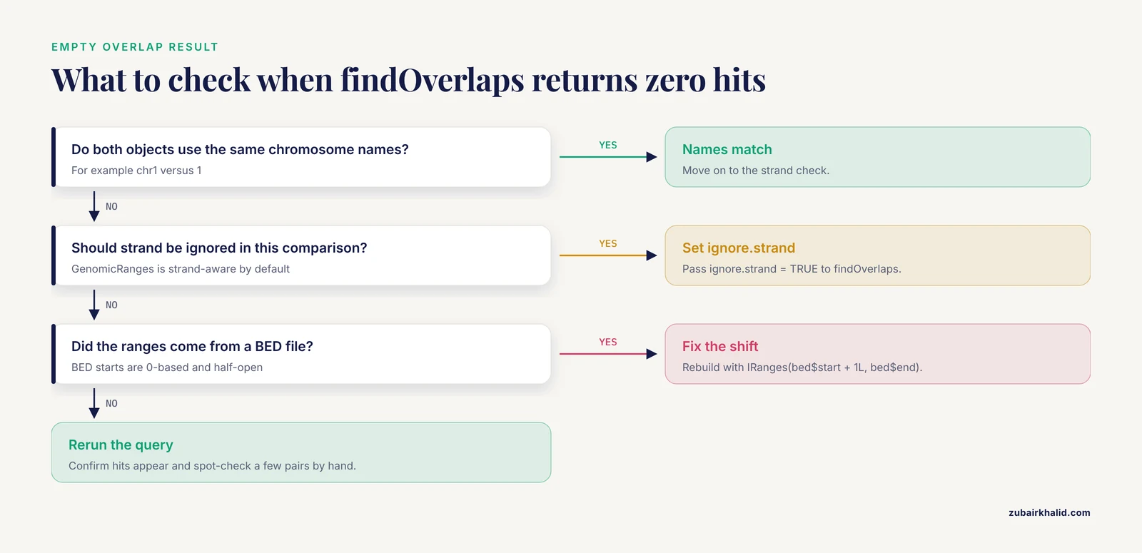
The most common causes are mismatched chromosome naming styles, such as chr1 versus 1, strand mismatch when the default strand-aware comparison is in effect, and a BED off-by-one error that shifted one set of ranges. Normalize seqlevels on both objects first with seqlevelsStyle or manual renaming.
What is the difference between union and punion?
union treats each argument as a whole set of positions and returns the merged union, while punion combines ranges pairwise and requires equal-length inputs. Use union for genome-level merging and punion when two objects correspond row by row.
Can IRanges handle chromosome and strand information?
No. A bare IRanges object has no chromosome names and no strand, so overlaps between ranges on different chromosomes will be counted as genuine. Build GRanges objects as soon as your data represents real genomic loci.
Next Steps
Once the IRanges layer is comfortable, three directions pay off quickly. First, learn the GenomicRanges accessors for seqnames, strand, and mcols, since every IRanges operation carries over. Second, learn rtracklayer for importing and exporting BED, GFF, and bigWig files directly as GRanges, which removes the manual coordinate conversion from your code. Third, when you need biological interpretation rather than arithmetic, move to annotation and enrichment tooling. Genomic interval analysis exists because NGS platforms produce loci representing variants, transcription factor occupancy, and histone marks, and those loci only become interpretable when compared against curated genomic and epigenomic annotation libraries [1]. Tools such as GLANET provide that annotation layer with sampling-based enrichment testing that adjusts for GC content and mappability, and they allow users to extend the built-in library with custom gene sets and genomic intervals of their own [1]. The interval operations you practiced here are the computational substrate under all of it, so time spent mastering IRanges compounds across your entire r for bioinformatics toolkit.