How to Interpret Single-Cell RNA-seq Clustering Results in R
By Dr. Zubair Khalid, DVM, MS, PhD ·

Interpreting single-cell RNA-seq clustering results means assigning biological meaning to the groups of cells that an algorithm placed together based on transcriptomic similarity. In R, it means opening the cluster assignments stored in a Seurat or SingleCellExperiment object, testing them against marker genes and differential expression, and deciding which clusters represent cell types, cell states, or artifacts.
This step matters because the clustering algorithm knows nothing about biology. It partitions cells into groups because you asked it to, using parameters you chose, on a reduced representation you built. The cluster labeled "7" in your DimPlot is not a cell type until evidence says so, and even then the label is a hypothesis rather than a fact. A systematic benchmark of 465 computational pipelines in cancer studies found that pipelines with similar clustering agreement can report very different marker gene sets, a discrepancy invisible to the metrics most analysts check [1]. Interpretation, not clustering itself, is where most scientific error enters a single-cell analysis. This article explains, step by step, how to read clustering output in R, how to validate it, and how to avoid the failure modes that reviewers of single-cell papers see most often.
What You Are Actually Looking at Inside the R Object
Before you interpret anything, you need to know where the interpretation targets live. In r for bioinformatics practice, almost every workflow ends in one of two container objects.
Seurat objects store clustering in the meta.data data frame and the active.ident slot. When you run FindClusters(), Seurat writes a column such as RNA_snn_res.0.5 (clustering at resolution 0.5 on the RNA assay's shared nearest neighbor graph) and a convenience column seurat_clusters.
library(Seurat)
pbmc <- RunPCA(pbmc, verbose = FALSE)
pbmc <- FindNeighbors(pbmc, dims = 1:10)
pbmc <- FindClusters(pbmc, resolution = 0.5)
pbmc <- RunUMAP(pbmc, dims = 1:10)

head([email protected][, c("seurat_clusters", "RNA_snn_res.0.5")])
DimPlot(pbmc, label = TRUE) + NoLegend()
SingleCellExperiment objects, the standard container in the Bioconductor ecosystem, store cluster labels as a column of colData. The bluster package provides the clustering algorithms, and scran and scater provide normalization, feature selection, and visualization.
library(scran)
library(scater)
library(bluster)

sce <- logNormCounts(sce)
dec <- modelGeneVar(sce)
top <- getTopHVGs(dec, n = 2000)
sce <- runPCA(sce, subset_row = top)
g <- buildSNNGraph(sce, k = 10, use.dimred = "PCA")
colLabels(sce) <- cluster_fast_greedy(g)
sce <- runUMAP(sce, dimred = "PCA")
plotReducedDim(sce, dimred = "UMAP", colour_by = "label")
Three components of either object carry interpretive weight:
- Cluster labels. Integer identifiers with no inherent meaning. They are renumbered whenever you change resolution or recluster, so a cluster called "3" in one run may be "5" in the next.
- Reduced dimensions. The PCA embedding (used for graph building) and the UMAP or t-SNE embedding (used for pictures only). UMAP coordinates are computed on a small number of principal components, typically the top 10 to 50, and the distances between cells in a UMAP plot are not reliable quantitative distances.
- Metadata columns. Percent mitochondrial reads, cell cycle scores, batch labels, sample of origin. These are your first checks when you ask whether a cluster is biological or technical.
A useful mental model is that clustering output is a coordinate system you impose on the data. Interpretation is the process of mapping known biology onto that coordinate system and checking whether the mapping holds.
Terms Most Often Confused When Reading Clustering Output
| Term | What it actually means | Commonly confused with |
|---|---|---|
| Cluster | A group of cells connected densely in a nearest neighbor graph at one resolution setting | Cell type, which requires orthogonal evidence |
Resolution (resolution in Seurat, k and cluster function in bluster) | A tuning knob for how many communities the graph algorithm splits into | Number of principal components, a separate choice |
Number of PCs (dims = 1:10) | How much of the variance structure feeds the graph | The number of clusters you will get |
| UMAP plot | A two-dimensional visualization of local neighbor structure | A quantitative map of cell-to-cell distances or a clustering result |
| Marker gene | A gene enriched in one cluster relative to the rest | A validated cell-type marker, or a causal driver |
| Differentially expressed gene | A gene whose abundance differs between defined groups of cells | A marker, though the terms overlap in practice |
| Cell state | A position along a continuous biological program, such as activation or maturation | A discrete cluster, which can split or merge a continuum artificially |
| Annotation | A biological label assigned to a cluster using markers, references, or prior knowledge | The clustering itself, which is unsupervised and label-free |
The Interpretation Workflow, Step by Step
Step 1: Rule out technical structure before naming anything
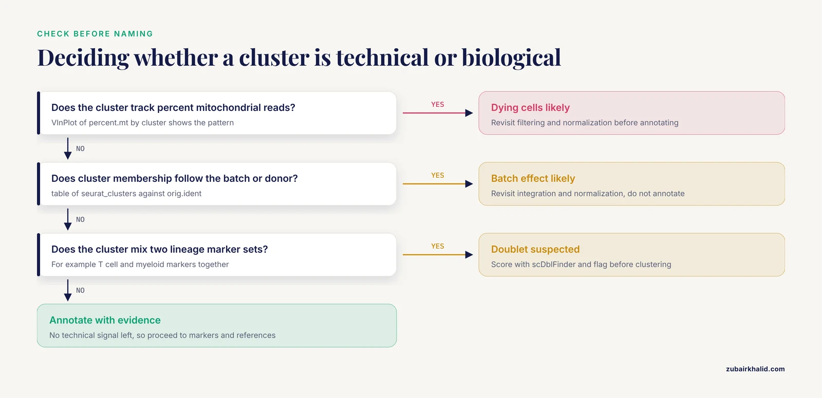
The first question about any cluster is whether it reflects biology. Cluster membership that correlates strongly with percent mitochondrial reads, cell cycle score, sequencing batch, or sample handling usually does not. In R, this check is cheap:
VlnPlot(pbmc, features = c("percent.mt", "nFeature_RNA"), group.by = "seurat_clusters")

# Chi-square or logistic association between cluster and batch
table(pbmc$seurat_clusters, pbmc$orig.ident)
If one cluster is essentially a batch, the correct response is to revisit integration and normalization rather than to annotate the cluster. If a cluster tracks the cell cycle, you decide deliberately whether proliferation is part of the biology you care about, and you document that decision, because it will shape every downstream comparison.
Doublet detection deserves a separate check. Clusters that contain a mixture of T cell and myeloid markers often are doublets, two cells captured in one droplet, rather than a rare transitional population. Tools such as scDblFinder (Bioconductor) score each cell and flag likely doublets before clustering, which prevents an artifact from entering your annotation table.
Step 2: Interrogate resolution and graph parameters
Clustering at a single resolution gives one view. The community-detection algorithms used in standard pipelines (Louvain and Leiden over a shared nearest neighbor graph) partition the graph at whatever granularity you request, and both the number of clusters and the membership of individual cells shift as you turn the knob [2]. Because the number of detected cell types varies substantially with the dimension reduction method and the clustering parameters, treating any single resolution as ground truth is unsupported [2].
In practice, scan a resolution range and compare:
resolutions <- c(0.2, 0.4, 0.6, 0.8, 1.0, 1.5)
for (r in resolutions) {
  pbmc <- FindClusters(pbmc, resolution = r)
}
# Examine how clusters split as resolution rises
table(pbmc$seurat_clusters, pbmc$RNA_snn_res.1.5)
When tracking how clusters divide across resolutions, the clustree package shows which clusters at low resolution give rise to which clusters at high resolution. A cluster that splits cleanly into two well-supported subclusters at higher resolution is a candidate real subpopulation. A cluster that reshuffles its cells chaotically between resolutions is unstable, and any annotation assigned to it should be held loosely.
The Bioconductor bluster package adds internal validity metrics so that stability is measured rather than eyeballed:
library(bluster)
clust.sil <- silhouette(as.integer(colLabels(sce)), dist(reducedDim(sce, "PCA")[, 1:10]))
summary(clust.sil$widths)
The silhouette width ranges from -1 to 1, where values near zero indicate cells sitting between clusters. Silhouette values summarize geometry only, and a good geometric score does not confirm biology, but poor values flag clusters worth a second look.
Step 3: Identify marker genes and read them critically
Marker discovery is the core interpretive move. In Seurat:
markers <- FindAllMarkers(pbmc,
  only.pos = TRUE,
  min.pct = 0.25,
  logfc.threshold = 0.25)
markers %>%
  group_by(cluster) %>%
  slice_max(n = 5, order_by = avg_log2FC)
Then visualize candidates on the embedding and across clusters:
VlnPlot(pbmc, features = c("MS4A1", "CD3E", "LYZ"), stack = TRUE, flip = TRUE)
FeaturePlot(pbmc, features = c("CD8A", "GNLY"))
DotPlot(pbmc, features = marker_panel, dot.scale = 8) + RotatedAxis()
Two interpretive caveats apply. First, a top-ranked cluster marker is a gene expressed preferentially in that cluster relative to all others. It is not automatically a canonical marker, and it is not automatically differentially expressed in the statistical sense you need for condition comparisons, because single-cell differential expression between clusters within a sample confounds cell type with donor. Pseudobulk aggregation per sample and cluster, then standard bulk-style testing across samples, is the design many analysts treat as the reference standard for between-condition differential expression. Second, genes can be non-randomly distributed in expression space without any cluster boundary separating them. The singleCellHaystack package finds genes expressed in cell subsets that occupy non-random positions in a multidimensional space using Kullback-Leibler divergence, without requiring a clustering at all, and it was designed precisely because how clusters are defined shapes which genes downstream analysis recovers [3]. Running a clustering-independent screen alongside FindAllMarkers is a low-cost way to check that your cluster boundaries are not hiding structure that the data contain.
Step 4: Annotate with multiple converging lines of evidence
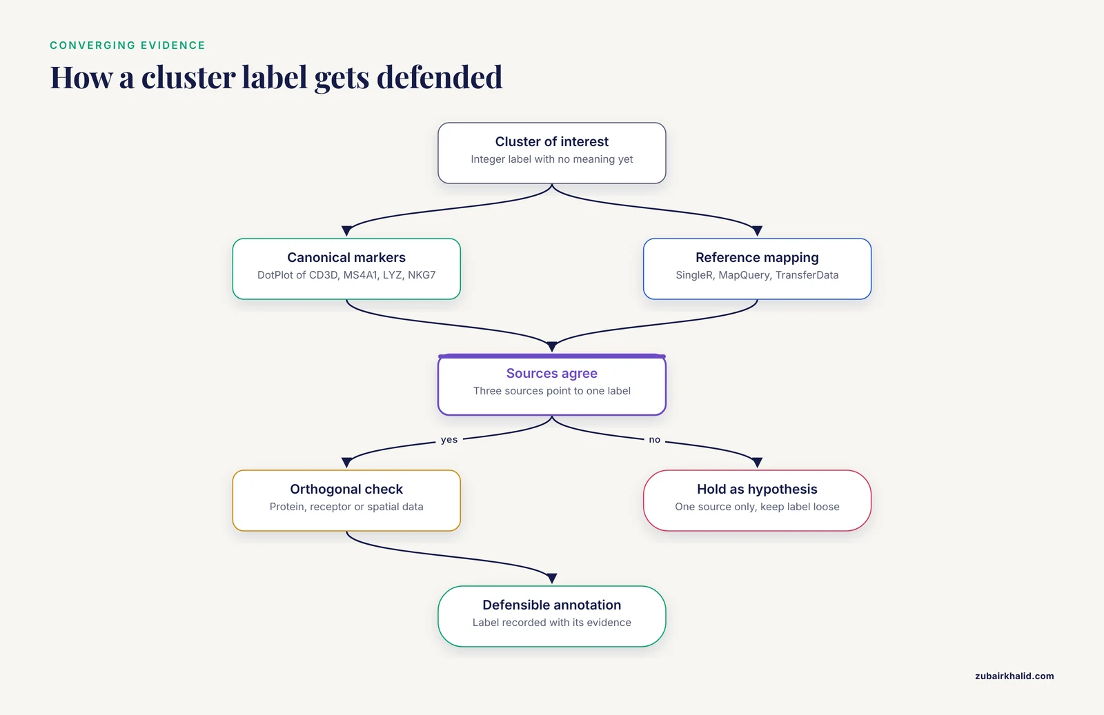
Annotation options, in rough order of reliability when used together:
- Canonical marker panels. For peripheral blood mononuclear cells, CD3D and CD3E for T cells, MS4A1 and CD79A for B cells, LYZ and S100A8 for monocytes, NKG7 and GNLY for natural killer cells. A
DotPlotacross clusters is the fastest way to see the pattern. - Reference mapping.
SingleR(Bioconductor) labels each cell against a curated reference. Seurat'sMapQueryandTransferDatamove labels from a reference atlas onto your data. For immune work, reference atlases built with surface protein validation are preferable, because protein measurements give a ground truth that transcriptome-only clustering lacks [4]. - Automated knowledge-guided tools. CLUEY integrates prior biological knowledge into the clustering process itself, guiding the number of clusters and improving the interpretability of the resulting groups across unimodal and multimodal datasets [2].
- Functional interpretation pipelines. ASURAT performs clustering and biological interpretation simultaneously, decomposing functional gene sets into terms covering cell type, disease, biological process, and signaling pathway, which adds an annotation layer that conventional gene-based analysis does not provide [5]. Latent Dirichlet allocation based methods take a related approach, estimating latent functions from raw count data in a cell-function-gene framework and producing biologically grounded cluster interpretations [6].
A single annotation source is a hypothesis. Three sources that agree is an annotation you can defend.
Step 5: Match granularity to the biological question
A recurring failure mode is annotating at the wrong granularity. If your question is "which immune compartments are present," eight major clusters suffice. If your question is "which macrophage activation programs associate with treatment response," eight clusters are far too coarse. Two tools address this directly.
Metacells. SEACells identifies metacells, groupings of cells that represent highly granular, distinct cell states, overcoming single-cell sparsity while retaining heterogeneity that traditional clustering obscures, and it works in both RNA and ATAC modalities across discrete and continuous (trajectory) datasets [7]. Metacells sit between single cells and clusters, which makes them useful when you want per-state summaries without forcing a continuum into discrete bins.
Gene programs. Non-negative matrix factorization decomposes expression into programs that can cut across cluster boundaries. In a renal cell carcinoma analysis of 443,337 cells, NMF identified interpretable gene programs within tumor-associated macrophage populations that related to immune checkpoint inhibitor response, structure that a static cluster label alone would not surface [8]. If a program of interest spans two clusters, that is a finding about biology, not an error in your clustering.
Step 6: Validate against data the transcriptome did not produce
The strongest validation comes from modalities that measure something other than RNA.
Surface protein and multimodal integration. Weighted-nearest neighbor analysis learns, for each cell, the relative utility of each modality, enabling integrative clustering of CITE-seq data (paired RNA and antibody-derived tags) and the construction of multimodal reference atlases that resolved subpopulations RNA-only analysis did not reveal [9]. The Orthogonal Multimodality Integration and Clustering method extends this idea by integrating multiple modalities while accounting for dependence among them, improving accuracy and interpretability on CITE-seq datasets [10]. When RNA clustering and protein staining disagree on a cluster, the disagreement is information, and the protein usually wins for lineage assignment.
Immune receptor data. For T and B cell studies, scRepertoire couples transcriptomic clustering with T cell receptor and immunoglobulin sequences from 10x Genomics immune profiling, so clonal relationships can confirm or overturn clusters that look similar transcriptionally [11].
Spatial context. A cluster annotation gains credibility when the cells occupy a coherent tissue location. Voyager brings exploratory spatial data analysis and geospatial statistics to single-cell data in both R/Bioconductor and Python, and its workflows demonstrate how spatial autocorrelation methods can reveal biologically relevant structure beyond what cluster geometry in an embedding shows [12]. Reviews of single-cell genomics in neuroscience make the same point at a field level: cell-intrinsic state and interactions between cell types are two distinct axes of variation, and spatially resolved methods are needed to address the second [13].
Step 7: Connect clusters back to samples and populations
Cluster interpretation does not end at the plot. The composition question, meaning how the abundance of each cluster changes across donors or conditions, is often the actual scientific question.
Cell composition analysis. Cell Population Mapping uses reference single-cell profiles to infer the composition of cell types and cell states from bulk transcriptome data through the scBio R package, and its application to influenza-infected mouse lungs showed that the relationship between cell abundance and clinical outcome can be a cell-state-specific property varying gradually along an activation continuum [14]. That result carries a direct interpretive lesson: a cluster annotation can hide a graded state axis, and bulk deconvolution against single-cell references can recover it.
Sample-level trajectories. PILOT computes Wasserstein distances between individual single-cell samples, representing each sample as its composition of cell clusters, enabling unsupervised identification of sample trajectories and cellular clusters associated with disease progression across cohorts of hundreds of samples [15]. Under this framing, a cluster matters not just for what its markers are but for how its abundance moves along a disease trajectory.
Why Clusters Are Not Cell Types: The Evidence
The most consequential misunderstanding in this field is the assumption that clustering recovers cell types by construction. Evidence says otherwise. In the Rhesus Immune Reference Atlas, transcriptional profiles were contrasted against immune lineages using surface protein and marker genes as ground truth, and the pattern of clustering aligned with cell type only sometimes. Within T and natural killer cell compartments, many functionally distinct subsets lacked defining markers, and strong shared expression programs such as cytotoxicity caused systematic intermingling of distinct subsets in unsupervised clustering [4]. The authors of that atlas concluded that directly measuring diagnostic gene programs complements unsupervised analysis rather than trusting the cluster structure alone [4].
Three consequences follow for anyone learning to interpret single cell clustering results:
- Clusters often split one continuous cell type along technical or activity gradients, or merge biologically distinct types that share a dominant program.
- Intermingling is systematic, not random, so it will reproduce across datasets and look convincing in a UMAP plot.
- The fix is orthogonal measurement, meaning protein panels, receptor sequencing, spatial validation, or diagnostic multi-gene signatures computed directly on the cells.
How Pipeline Choices Change What You See
Every interpretive conclusion is conditional on the pipeline that produced it. The scale of this effect was quantified in a benchmark that tested combinations of 5 normalization methods and 4 clustering algorithms across 3 cancer datasets with more than 434,000 cells, using a Biological Discordance Score that measures how marker gene interpretation changes across pipelines. Normalization method choice had a greater impact on biological interpretation than clustering algorithm selection, and pipelines with similar clustering agreement could identify up to 86 percent different marker genes. Log-normalization showed the best balance of performance and interpretive stability across the cancer types tested [1].
For the analyst, this changes what a marker gene list means. The genes in your FindAllMarkers table are markers of clusters under one normalization, one feature selection, one set of dimensions, and one graph. Robust conclusions are those that survive a sensitivity check, for example re-running the pipeline with a second normalization or a second dimensionality setting and confirming that the annotation, not merely the cluster count, holds. Deep generative frameworks such as inClust take a complementary route, embedding auxiliary information and supporting supervised, semi-supervised, or unsupervised modes so that labels and covariates constrain the decomposition [16], and graph attentional methods such as scGAC learn clustering-friendly representations by propagating information across cells with learned weights [17]. Benchmarking studies of these newer methods generally report gains over earlier baselines on real datasets, but the practical implication for interpretation is the same in every case, meaning you must know which algorithm touched your labels and under what settings.
A Worked Example: Reading a PBMC Clustering Result
Consider a standard 10x Genomics PBMC dataset clustered in Seurat. You obtain nine clusters. The interpretation sequence looks like this:
VlnPlotshows percent mitochondrial reads is flat across clusters, and the chi-square table shows clusters distributed evenly across two donors. No obvious technical cluster.- Resolution 0.4 gives seven clusters, 0.8 gives nine, 1.2 gives twelve. Clusters 0, 1, and 2 at 0.8 each split cleanly at 1.2, and
clustreeshows clean bifurcation rather than churn. FindAllMarkersreturns CD3D, CD3E, IL7R for cluster 0, MS4A1, CD79A for cluster 2, LYZ, S100A9, FCGR3A separated into two myeloid clusters, and PPBP plus PF4 in a small cluster 8.- The PPBP/PF4 cluster is a known platelet contamination artifact in droplet datasets, not a tissue population. You annotate it as platelets and report it as such, or exclude it, documenting the choice.
- The two myeloid clusters separate on FCGR3A (CD16) versus CD14, which maps to classical and non-classical monocytes.
SingleRagainst a reference agrees. - You notice NKG7 high in both a CD3D-positive cluster and a CD3D-negative cluster. You check protein tags if available or receptor data with scRepertoire, and you decide whether the CD3D-positive NKG7-high group is a real cytotoxic T population or intermingling of a shared cytotoxicity program [4].
Nine clusters in, nine annotated entities out, with one artifact identified and one ambiguity flagged rather than silently resolved. That is what a defensible interpretation looks like on the record.
Common Mistakes and Limitations
Reading UMAP geometry as data. Cells that appear adjacent in a UMAP plot are neighbors under the specific projection parameters you used, and distant-looking groups can be biologically closer than they appear. Cluster identity claims should rest on markers, graph connectivity, and validation, never on the shape of the plot.
Fixing resolution by habit. Running everything at resolution 0.4 because a tutorial did is not a decision. Because the detected number of cell types varies with dimension reduction and clustering parameters, resolution should be scanned and the choice justified against the biological question [2].
Annotating the biggest marker per cluster. The single top gene by log fold change is frequently a stress, dissociation, or cell cycle gene. Read the top 20 markers as a pattern, and cross-check against canonical panels.
Confusing cluster markers with condition DEGs. Differential expression between clusters within one donor answers a different question than differential expression between disease states. Use pseudobulk per sample for condition-level claims.
Ignoring normalization sensitivity. Marker gene lists can differ substantially between pipelines with similar clustering agreement, so conclusions built on one normalization should be spot-checked against another [1].
Trusting unsupervised structure over orthogonal ground truth. Functionally distinct T and NK subsets can intermingle in transcriptome-only clustering because of shared programs such as cytotoxicity, so protein, receptor, or program-level measurements are needed where lineage definitions matter [4].
Forcing continuous states into discrete labels. Activation continua can vary gradually across cells, and assigning one label to the whole range erases the gradient that may carry the biological signal [14]. Metacells or gene program analyses preserve that granularity better than hard clusters [7].
Skipping the artifact sweep. Platelet contamination, doublets, high-mitochondrial dying cells, and batch effects all produce clusters that look like biology. Check them before annotation, every time, on every dataset.
Quick Review
- A cluster is a graph partition at one resolution setting, not a cell type. Annotation is a separate, evidence-based act.
- Check mitochondrial content, cell cycle, batch, and doublet scores before naming any cluster.
- Scan resolution across a range and use tools like
clustreeand silhouette scores to judge stability rather than picking a default. - Read markers as patterns with
DotPlotandFeaturePlot, and complement cluster-based tests with clustering-independent screens such as singleCellHaystack [3]. - Pipeline choices, especially normalization, can change marker gene interpretation dramatically even when clustering agreement looks similar [1].
- Validate with orthogonal data, meaning surface proteins through multimodal integration [9], immune receptors through scRepertoire [11], or spatial context through tools like Voyager [12].
- For continuous biology, use metacells [7] and gene programs [8] alongside, or instead of, hard cluster labels.
Frequently Asked Questions
What does it mean to interpret single-cell RNA-seq clustering results?
It means assigning and validating biological meaning, such as cell type, cell state, or artifact, to the groups of cells produced by a clustering algorithm. The cluster labels themselves are arbitrary integers, and interpretation is the evidence-based process of mapping markers, references, and orthogonal data onto them.
Which R packages should I use for clustering and interpretation?
Seurat and the Bioconductor stack of scran, scater, and bluster are the two standard ecosystems, and both store cluster labels in well-defined slots you can inspect programmatically. Complementary packages include singleCellHaystack for clustering-independent gene detection [3], scRepertoire for immune receptor integration [11], and knowledge-guided frameworks such as CLUEY [2] or ASURAT [5] when you want interpretability built into the clustering step.
Do clusters in a UMAP plot correspond directly to cell types?
No. Clusters often align with cell types but not always, and functionally distinct subsets can intermingle when they share dominant expression programs, a pattern documented experimentally in T and NK cells using surface protein ground truth [4]. Use the UMAP for visualization and rely on markers and orthogonal validation for labels.
How do I choose the right resolution for clustering?
Scan a range of resolutions, examine how clusters split using a tree visualization, and check marker coherence at each level against your biological question. Because the number of detected cell types depends on dimension reduction and clustering parameters, no single resolution is inherently correct [2], and the choice should be reported and justified rather than defaulted.
Why do my marker genes differ from another published analysis of the same tissue?
Different normalization methods, feature selection, dimensionality settings, and clustering algorithms produce different marker lists even when the clusters look similar, with benchmarking showing large marker discordance invisible to standard agreement metrics [1]. Compare pipelines at the level of annotations and robust conclusions rather than expecting identical gene tables.
Can I use clustering results to compare cell proportions across patients?
Yes, but treat clusters as one level of resolution on cell states. Composition methods such as Cell Population Mapping use single-cell references to infer cell type and state proportions from bulk data [14], and sample-level frameworks such as PILOT compute distances between patients based on their cluster compositions to find disease-associated trajectories [15]. Keep in mind that graded state continua within an annotated cluster can carry the real signal.
Sources
- Normalization choice drives biological interpretation in single-cell RNA-seq cancer studies: A systematic benchmarking of 465 computational pipelines
- CLUEY enables knowledge-guided clustering and cell type detection from single-cell omics data
- A clustering-independent method for finding differentially expressed genes in single-cell transcriptome data
- Enhanced interpretation of immune cell phenotype and function through a rhesus macaque single-cell atlas
- ASURAT: functional annotation-driven unsupervised clustering of single-cell transcriptomes
- An interpretable single-cell RNA sequencing data clustering method based on latent Dirichlet allocation
- SEACells infers transcriptional and epigenomic cellular states from single-cell genomics data
- Investigation of tumor-associated macrophages (TAMs) and therapeutic resistance to immune checkpoint inhibitors (ICI) through single-cell analysis of renal cell carcinoma (RCC).
- Integrated analysis of multimodal single-cell data
- Orthogonal multimodality integration and clustering in single-cell data
- scRepertoire: An R-based toolkit for single-cell immune receptor analysis
- Voyager: exploratory single-cell genomics data analysis with geospatial statistics
- Opportunities and challenges of single-cell and spatially resolved genomics methods for neuroscience discovery
- Cell composition analysis of bulk genomics using single cell data
- Detection of PatIent-Level distances from single cell genomics and pathomics data with Optimal Transport (PILOT)
- A deep generative framework with embedded vector arithmetic and classifier for sample generation, label transfer, and clustering of single-cell data
- scGAC: a graph attentional architecture for clustering single-cell RNA-seq data