How to Interpret Bioinformatics Results in Biological Context
By Dr. Zubair Khalid, DVM, MS, PhD ·

Interpreting bioinformatics results in biological context means reading a computational output, such as a list of differentially expressed genes or an enriched pathway, as a claim about cells, tissues, or organisms rather than as a standalone statistic. A complete interpretation states what the result says about the biological system, the conditions under which that claim holds, and the independent evidence needed before the claim becomes accepted biology.
A table of p-values contains no biology by itself. The same upregulated gene list can mean that a disease altered gene regulation, that the diseased samples simply contained more of a different cell type, or that samples handled in a different sequencing batch behaved differently. Published studies show how sharply context can change conclusions. In a study linking type 2 diabetes to atherosclerosis, the two strongest candidate genes showed reproducible but disease-context-dependent expression across datasets [1]. In head and neck squamous cell carcinoma, a prognostic gene signature became coherent only after the researchers built smoking background into the discovery design itself [2]. In inflammatory bowel disease, the authors deliberately limited their claims to what the measurement could support, describing cross-sectional participant-level organization rather than receptor activation [3]. Attaching context to numbers is a learnable skill, and this article teaches it as a set of concrete habits you can apply to your own output files.
What Does Interpreting Results in Biological Context Actually Mean?
Students who ask what the phrase means usually want a rule they can apply immediately. The rule has three parts, and every defensible interpretation contains all three.
The three parts of a contextual interpretation
Part 1: The statistical result, stated precisely. Name the test and the quantity. "CD74 has an adjusted p-value of 0.004 and a log2 fold change of 1.8 in ileal Crohn disease biopsy tissue versus healthy control tissue" is a precise statement. "CD74 is upregulated in inflammation" is not, because it drops the comparison, the tissue, and the effect size.
Part 2: The biological frame. This is the mapping from the measurement to the system. The measured quantity here is bulk mRNA abundance averaged across every cell in the biopsy. The frame asks which cell populations, pathways, and known mechanisms could produce that averaged signal. A frame can invalidate a tempting conclusion. If immune cells infiltrated the diseased tissue, an immune gene can rise without any per-cell regulatory change.
Part 3: The evidence boundary. State what the analysis cannot establish. A cross-sectional association cannot establish a time course. An enrichment result cannot establish that a pathway is activated. A hub gene ranking cannot establish causality. Writing the boundary down, in one sentence, is the habit that separates careful interpretation from overclaiming.
Summary table: what each common result states, and what it does not
| Result you see | What it literally states | What it does not state | Context question to ask |
|---|---|---|---|
| Adjusted p-value (FDR) of 0.003 | The observation is unlikely under the null hypothesis, with an estimated false discovery rate of about 0.3 percent across rejected tests | Nothing about effect size, mechanism, or cause | How large is the effect, and does it replicate in an independent cohort? |
| log2 fold change of 2.1 | The measured abundance roughly quadrupled between the two compared groups | Nothing about why, or whether the change drives disease | Which cell types and conditions produced this change? |
| Enriched Gene Ontology term, FDR 0.01 | Genes sharing this annotation appear in your list more often than expected by chance | Nothing about direction of change or pathway activity | Did the contributing genes go up or down, and is the annotation direct or inferred? |
| GSEA normalized enrichment score of 1.8 | The gene set sits toward one end of your ranked list more than random gene sets do | Nothing about which genes drive the signal | Where is the leading edge, and does its direction match the differential expression? |
| Module eigengene correlated with a trait | The module's average expression pattern tracks the trait across samples | Nothing about causation or which genes inside the module matter | Does the module replicate, and do its hub genes hold up experimentally? |
| Hub gene from cytoHubba MCC ranking | The gene's node in a protein interaction network ranks highly by maximal clique centrality | Nothing about its role in your disease or tissue | Is the interaction evidence relevant to this tissue, and has the gene been perturbed experimentally? |
Two definitions keep recurring in that table. The false discovery rate (FDR) is the expected proportion of false positives among the results you call significant, usually controlled with the Benjamini-Hochberg procedure. The log2 fold change is the base-2 logarithm of the ratio of mean expression between groups, so a log2 fold change of 1 means a doubling and 2 means a quadrupling.
How to Interpret Bioinformatics Results in Biological Context, Step by Step
Most interpretation errors are made at fixed points in a standard pipeline. Walking the pipeline with interpretation checkpoints makes those points visible. The steps below describe a bulk RNA-seq or microarray workflow, the most common setting in which students first learn bioinformatics.
Step 1. Define the biological question and the comparison before computing
Decide the contrast first: disease versus control, smoker versus never-smoker, tumor versus adjacent normal, treated versus untreated. Write down the confounders you already know about, such as age, sex, smoking status, medication, tissue composition, and batch. Every later interpretation inherits the quality of this decision. A comparison defined after seeing the results is a fishing expedition, and it should be labeled as one.
Step 2. Quality control and preprocessing
Run FastQC on raw sequencing reads, align or quantify with a standard tool such as STAR or Salmon, and inspect sample clustering before any differential test. A principal component plot that separates samples by sequencing date rather than by disease is telling you the dominant signal in your data is batch, not biology. Batch effects are systematic technical differences between processing groups. You cannot interpret a disease signal that co-occurs with a batch signal unless the design lets you separate them statistically.
Step 3. Differential expression testing
For microarray data and many RNA-seq designs, the limma R package is the standard linear model tool, with empirical Bayes moderation that stabilizes variance estimates across genes. A minimal, standard analysis looks like this:
library(limma)
design <- model.matrix(~ 0 + group)
fit <- lmFit(expr_matrix, design)
fit <- eBayes(fit)
results <- topTable(fit, coef = "Disease_vs_Control",
                    number = Inf, adjust.method = "BH")
This is exactly the class of analysis used to identify differentially expressed genes in published dataset comparisons such as the diabetes and atherosclerosis study discussed below [1]. The interpretation checkpoint here is the design matrix. The model.matrix line encodes which comparison the p-values describe, and any covariates you omit are confounded with the group effect.
Step 4. Multiple testing correction and effect sizes
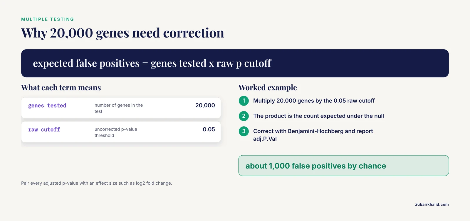
Testing 20,000 genes at a raw p-value cutoff of 0.05 will produce about 1,000 false positives by chance. Correct for this with Benjamini-Hochberg FDR, reported in limma output as adj.P.Val. Then apply a minimum effect size, commonly an absolute log2 fold change above 1, while understanding that the threshold is a convention, not a law of nature. Report both numbers for every gene you highlight. A gene with FDR of 1e-12 and a log2 fold change of 0.05 is statistically rock solid and biologically trivial in most contexts.
Step 5. Enrichment analysis
Convert the gene list into pathway-level statements. The two standard approaches, over-representation analysis and gene set enrichment analysis, are covered in detail in the next section, and the clusterProfiler R package implements both with a documented workflow from testing through network visualization [4].
Step 6. Modules, networks, and integration
Cluster genes by co-expression into modules, map proteins into interaction networks, and overlay your statistics onto both. These methods prioritize candidates and reveal structure that single-gene lists hide, but they add their own assumptions, covered in the networks section below.
Step 7. Validation and triangulation
Replicate in independent datasets, test the signature's discriminatory performance, and where possible perturb the leading candidates experimentally. Interpretation is strongest when statistical, computational, and experimental lines of evidence converge, a principle illustrated by both worked examples below.
Reading a Differential Expression Table
Open any limma, DESeq2, or edgeR output and you will see the same core columns. Learn them once and you can read most papers.
- Gene identifier. Prefer stable identifiers such as Ensembl IDs during analysis, and map to symbols only for display, because symbols are ambiguous.
- log2FC. The effect size and the number you should quote first.
- AveExpr. The average abundance. Low-abundance genes produce unstable fold changes.
- t and P.Value. The test statistic and its uncorrected probability.
- adj.P.Val. The FDR-adjusted value, and the number that determines your gene list.
A volcano plot displays log2 fold change on the x-axis against negative log adjusted p-value on the y-axis. Points in the upper right are significantly upregulated, upper left significantly downregulated. When you read one, ask three questions. How many genes pass the stated thresholds? Are strong fold changes and strong significance correlated, as they should be in clean data? Do the labeled genes make sense for the tissue, or do they look like blood, stress-response, or housekeeping artifacts?
The most common student error at this stage is treating the thresholded list as the finding. The list is an input to interpretation. The finding is a pattern, such as "extracellular matrix genes shift coordinately in the diseased tissue", and patterns survive small changes in thresholds while individual gene lists often do not.
Enrichment Analysis: The Two Main Tests and How to Read Them
Functional enrichment analysis is the standard bridge between a gene list and biological meaning, and it is the point where interpretation matters most, because enrichment output is the easiest output to overread [4].
Over-representation analysis versus gene set enrichment analysis
| Feature | Over-representation analysis (ORA) | Gene set enrichment analysis (GSEA) |
|---|---|---|
| Input | A thresholded list, for example all genes with FDR below 0.05 | All genes ranked by a statistic, such as the moderated t value |
| Test | Hypergeometric or Fisher's exact test | A running sum statistic evaluated across the ranked list |
| Threshold dependence | Strong, the list cutoff defines the result | None at the gene level, though the ranking statistic matters |
| Directionality | Must be run separately on upregulated and downregulated genes | Encoded in the sign of the enrichment score |
| Best use | Interpreting a short curated list | Detecting coordinated, subtle shifts across a pathway |
ORA asks whether a set of genes sharing an annotation, for example a Gene Ontology (GO) biological process term, appears in your list more often than expected by chance, given the background. GSEA asks whether the genes of a set cluster toward one end of a fully ranked list. In clusterProfiler, a standard ORA call specifies the organism database, the ontology branch, and the correction method:
library(clusterProfiler)
ego <- enrichGO(gene          = upregulated_entrez_ids,
                OrgDb         = org.Hs.eg.db,
                keyType       = "ENTREZID",
                ont           = "BP",
                pAdjustMethod = "BH",
                pvalueCutoff  = 0.05)
Four interpretation rules for enrichment output
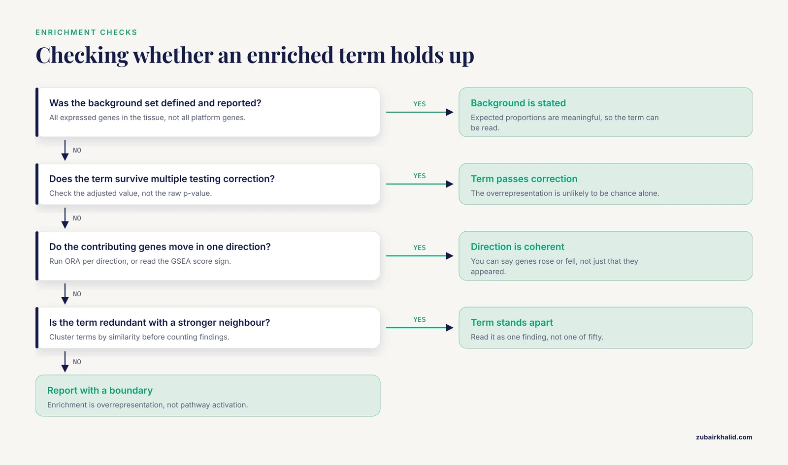
Rule 1: The background determines the answer. ORA is a comparison between your list and a background universe. If your background is all genes assayed on the platform rather than all expressed genes in the tissue, the expected proportions shift and so do the enriched terms. Always check and report the background.
Rule 2: Terms are redundant. GO terms form a hierarchy, and dozens of near-identical terms can pass the cutoff because they share most of their genes. Reading fifty terms as fifty findings is the classic beginner error. The practical fix is to compute similarity between enriched terms and cluster them, then read one cluster as one finding. A current protocol workflow does exactly this, performing ORA and GSEA with clusterProfiler, calculating term similarity between enriched terms, and exporting the resulting network to Cytoscape with the cyemapplot function for interactive exploration [4].
Rule 3: Direction is not optional. An enriched term says nothing about whether its genes went up or down unless you arranged for that information. Run ORA separately on upregulated and downregulated genes, or use GSEA where the sign of the score carries direction. Advanced network visualizations now integrate expression directionality directly into the display, so that a viewer can see whether a functional module is driven by upregulated genes, downregulated genes, or both [4].
Rule 4: Enrichment is not activation. "Oxidative phosphorylation enriched, FDR 0.001" does not mean oxidative phosphorylation sped up. It means the genes in that set are overrepresented in your list. Pathway activity requires directed reasoning, and where possible, evidence from other data layers.
Reading enrichment networks
Bar plots and dot plots summarize terms one at a time. Networks show relationships. In an enrichment map, each node is an enriched term and each edge reflects shared gene content, so functional modules appear as clusters of connected nodes. A recent protocol demonstrates three complementary styles: basic networks that reveal functional modules and term relationships, pie chart networks in which node properties quantify pathway coverage to help prioritize complete versus partial perturbations, and networks that integrate the direction of differential expression across genes in each term [4]. The interpretive payoff is prioritization. When hundreds of terms pass the cutoff, the network view tells you which clusters are distinct findings and which are one finding drawn many times.
Modules, Hubs, and Networks: What the Numbers Do and Do Not Say
Co-expression modules
Weighted gene co-expression network analysis (WGCNA) groups genes into modules based on correlated expression across samples. Each module is summarized by its eigengene, the first principal component of the module's expression matrix, which can be correlated with traits such as disease status. A correlation of 0.6 between a module eigengene and disease status means the module's average behavior tracks the disease across samples. It does not mean the module causes the disease, and it does not tell you which genes inside the module carry the signal. Both require further work.
Protein interaction networks and hub genes
A protein-protein interaction (PPI) network connects proteins whose physical or functional interactions are catalogued in public databases. Tools such as cytoHubba rank nodes with centrality measures, including maximal clique centrality (MCC), which favors proteins that participate in many fully connected neighborhoods, and MCODE detects densely connected subnetworks. GeneMANIA extends a seed network with additional predicted interactions. These tools are prioritization engines. A high MCC rank says a protein is well connected in the database, which partly reflects how thoroughly it has been studied. Well-studied proteins are overrepresented in interaction databases, so hub status can be partly a popularity artifact. Hub status becomes biology only when the gene's expression, replication, and experimental perturbation agree with the network story.
Learning what the algorithm actually computes
You cannot interpret a centrality score or a module detection output without knowing what the algorithm computes, and network methods are usually documented for a technical audience. Graphery, an interactive tutorial webserver, addresses this gap by pairing foundational graph concepts with executable Python code that runs directly on real biological networks, letting users modify the code and see the effect without creating an account [5]. If you are taking a bioinformatics course or teaching yourself, running a degree calculation or a community detection routine on a small network is the fastest way to understand what the numbers in your own analysis mean. Degree counts a node's direct connections. Betweenness counts how often a node lies on shortest paths between others. Modularity measures how cleanly a network splits into communities. Each of these, when reported about your data, is a statement about the graph you built, not automatically about the organism.
A Worked Example: Type 2 Diabetes and Atherosclerosis
A single published pipeline, followed end to end, teaches interpretation better than any abstract advice. A study of the molecular link between type 2 diabetes mellitus (T2DM) and atherosclerosis (AS) illustrates the full chain from public data to validated candidates [1].
The design came first. The authors used two public Gene Expression Omnibus (GEO) datasets as training data, GSE38642 for T2DM and GSE100927 for atherosclerosis, and held out two further datasets, GSE41762 and GSE57691, for validation. They identified differentially expressed genes with limma and disease-associated modules with weighted gene co-expression network analysis, then intersected the differentially expressed genes with module genes. That intersection is the interpretive heart of the design. A gene that is both statistically shifted and co-expressed with the disease program has two independent lines of computational evidence, which filters out single-method artifacts.
The candidates then passed through protein-protein interaction analysis, cytoHubba MCC ranking, and MCODE screening, followed by an unusually broad validation battery: expression validation, receiver operating characteristic (ROC) analysis, cross-validation, permutation testing, GeneMANIA network extension, GSEA, single-sample GSEA (ssGSEA) based immune infiltration analysis, regulatory network construction, and exploratory drug-gene enrichment [1]. ssGSEA quantifies the enrichment of immune cell signatures in each individual sample, which lets the authors ask whether immune composition, rather than gene regulation, explains part of the signal. ROC analysis measures how well a small gene panel separates diseased from healthy samples, summarized as the area under the curve.
The final step left the computer. Selected candidates were examined in mouse models. The result was twenty-one overlapping genes, six candidate hub genes, and, among them, two genes, C7 and MFAP4, with reproducible but disease-context-dependent expression patterns across the training and validation datasets [1]. Read that final phrase carefully, because it is a model of honest interpretation. The authors did not claim C7 and MFAP4 are "the genes causing diabetic atherosclerosis". They claimed reproducibility, they flagged context dependence, and they left the mechanistic claim to the experimental work. Every stage of this pipeline is a filter with assumptions, and the honest summary of a filtering pipeline is a short list of candidates, not a mechanism.
Context as a Design Variable, Not a Footnote
The strongest contemporary studies do not add context after the analysis. They build it into the design, and two recent examples show what that looks like in practice.
Smoking status in head and neck cancer
Tobacco exposure reshapes both the genome and the tumor microenvironment in head and neck squamous cell carcinoma (HNSCC), so a prognostic signature that ignores smoking may mix two signals. One study integrated single-cell RNA-seq with bulk RNA-seq from TCGA-HNSC, used smoking-background differential expression for candidate discovery, identified cancer-associated fibroblast (CAF) associated gene modules with hdWGCNA, a single-cell adaptation of co-expression network analysis, and constructed an 11-gene smoking-related CAF signature with machine learning [2]. The single-cell layer anchored the bulk signals to specific cell types. The researchers identified five transcriptionally distinct CAF subtypes, found that matrix-remodeling CAFs showed extracellular matrix features, and reported that higher MuSiC-inferred matCAF relative abundance was associated with poorer survival, where MuSiC is a deconvolution method that estimates cell-type proportions in bulk tissue from a single-cell reference [2]. They then evaluated the signature in external cohorts, examined it with immune deconvolution and SHAP-based feature interpretation, where SHAP is a game-theoretic method for attributing a model's predictions to its input features, and finally modulated INHBA expression in HNSCC cell lines to test effects on proliferation, migration, invasion, and epithelial-mesenchymal transition features [2]. The lesson for interpretation is structural. Because smoking entered at discovery, every downstream number, from module correlation to signature performance, means something specific about the smoking-relevant biology rather than about a mixture of smoker and never-smoker tumors.
Naming the measurement in inflammatory bowel disease
A study of inflammatory bowel disease (IBD) shows the third part of interpretation, the evidence boundary, executed deliberately. The authors analyzed Human Microbiome Project 2 (HMP2) mucosal transcriptomes at the participant level to test whether metabolite-sensing host programs covary with neuroimmune receptor-side programs, and they operationalized receptor-side neuroimmune remodeling as cross-sectional participant-level host-program organization together with compartmental localization of receptor transcripts, explicitly not as longitudinal change or receptor activation [3]. They then examined the stability of those relationships through diagnosis and inflammation adjustment, participant-grouped explanatory modeling, and tissue-composition sensitivity analyses, supported by complementary metabolomic and single-cell datasets [3]. Each of those choices is an interpretation safeguard. Adjustment asks whether the association survives confounding by diagnosis and inflammation. Tissue-composition sensitivity analysis asks whether the signal is really a cell-type proportion effect. And the operationalization sentence tells the reader exactly what the measurement is, so no one can later misread a cross-sectional covariance as a dynamic process. When you write up your own results, write that sentence.
Interpreting Simulation and Model-Based Results
Not all bioinformatics output is a table of genes. Agent-based and mechanistic simulations produce their own interpretation problems, and the discipline developed for them transfers directly to statistical models and machine learning signatures. Spartan, an R package of statistical techniques distributed through CRAN, was designed to help researchers establish the relationship between a computer simulation and the real biological system it models, and specifically to identify which simulation results are attributable to the dynamics of the modeled system rather than to artifacts of biological uncertainty, parametrization, or simulation stochasticity [6]. Its techniques include uncertainty and sensitivity analysis, in which parameters are varied systematically to see which ones drive the output, and stochastic replication, in which repeated runs of the same model reveal how much the output wobbles by chance. The package demonstrated this on lymphoid tissue development in the small intestine, showing which aspects of simulated behavior reflected the modeled biology and which reflected parameter choices [6].
The transferable habit is to ask, of any model output, whether the result survives perturbation of the things you are unsure about. If a co-expression module, a prognostic signature, or a simulated trajectory changes qualitatively when a reasonable alternative parameter or preprocessing choice is used, the result is fragile, and fragile results should not be interpreted as biology.
How Interpretations Are Tested in Practice
Interpretation earns confidence through triangulation, and the literature provides a clear hierarchy of tests.
- Computational replication. The same analysis in independent datasets, ideally from different laboratories and platforms. The diabetes and atherosclerosis study reserved two GEO datasets purely for this purpose [1].
- Discriminatory performance. ROC analysis with cross-validation and permutation testing, which asks whether a gene panel separates disease from health better than chance and better than an overfitted model would [1].
- Orthogonal inference. Immune deconvolution and ssGSEA ask whether cell composition explains the signal, and SHAP analysis opens a machine learning signature to see which features drive its predictions [1][2].
- Experimental perturbation. Changing a candidate gene in cells and measuring the consequence. The HNSCC study modulated INHBA in cell lines and measured proliferation, migration, invasion, and EMT-related features, converting a correlational candidate into a functional claim [2].
- Animal models. The diabetes and atherosclerosis candidates were examined in mouse models, the step that connects human dataset statistics to organism-level biology [1].
Each level answers a different objection. Replication answers "was it a fluke of one dataset". Deconvolution answers "is it just cell composition". Perturbation answers "does the gene do anything". Animal work answers "does it matter in a whole organism". An interpretation that has passed only the first level should be phrased as a hypothesis, and published papers that pass all five still describe their candidates as candidates.
Common Mistakes and Limitations
These are the errors that most often corrupt interpretation, drawn from the failure modes visible in real analyses.
- Quoting significance without effect size. An FDR of 1e-9 on a 0.04 log2 fold change is not a strong biological signal. Always pair the two numbers.
- Ignoring the ORA background. Using all platform genes instead of all expressed genes changes which terms appear enriched. Report the universe.
- Reading redundant terms as independent findings. Fifty overlapping GO terms are usually three findings. Cluster by term similarity before counting [4].
- Treating enrichment as pathway activation. Enrichment is overrepresentation in a list. Direction and activity require additional evidence [4].
- Trusting hub rankings as mechanism. Centrality in a public PPI network partly reflects how well studied a protein is. Hub status is a prioritization, validated only by perturbation experiments [1].
- Ignoring tissue composition. In bulk tissue, a cell-type proportion shift can masquerade as regulatory change. Deconvolution and composition sensitivity analyses exist precisely to catch this [2][3].
- Overfitting signatures. With small sample sizes and many features, machine learning will find structure in noise. External cohorts, cross-validation, and permutation testing are the minimum defenses [1].
- Interpreting cross-sectional associations as dynamics. Covariance across participants at one time point says nothing about trajectory or activation unless the design measured it [3].
- Ignoring batch and design. A disease signal that tracks a processing batch cannot be interpreted until the design separates them.
- Skipping the operationalization sentence. If you cannot state in one sentence what your key variable actually measures, you are not ready to interpret it.
A final limitation applies to the field as a whole. Individual datasets, especially those intended for clinical or experimental follow-up, benefit from review by a biostatistician or a domain specialist who knows the tissue and disease involved.
Quick Review
- Every computational result answers a statistical question. It answers a biological question only after you supply the frame, the conditions, and the evidence boundary.
- Report effect size with every p-value, and treat thresholds as conventions rather than truths.
- In ORA, the background gene set and the list cutoff jointly determine the result. In GSEA, the sign of the score carries direction.
- Enriched terms are redundant. Cluster them by similarity and read clusters, not individual terms [4].
- Context variables such as smoking status, inflammation, and tissue composition can explain an entire signal, so build them into discovery and test them with sensitivity analyses [2][3].
- Hub status, module membership, and signature scores are prioritizations. Replication, deconvolution, and experimental perturbation turn them into biology [1].
- Match your claims to your operationalization. A cross-sectional covariance is not a time course, and an enriched term is not an activated pathway [3].
Frequently Asked Questions
What does it mean to interpret bioinformatics results in biological context?
It means stating what a computational result says about the biological system, the conditions under which the statement holds, and what independent evidence would be needed to confirm it. A p-value, fold change, or enrichment score becomes an interpretation only when those three elements are attached.
What is the difference between statistical significance and biological significance?
Statistical significance measures how unlikely the observation is under a null hypothesis, while biological significance concerns the size and meaning of the effect in the organism. A result can be statistically unshakable and biologically trivial, so both the adjusted p-value and the effect size must be reported together.
How do I know whether an enriched pathway is real?
Check four things: that the background gene set was defined correctly, that the term survives correction for multiple testing, that the contributing genes move in a coherent direction, and that the term is not simply redundant with a stronger neighboring term. Clustering enriched terms by similarity and inspecting the leading-edge genes are the practical checks.
Should I trust hub genes from a protein interaction network?
Treat them as prioritized candidates, not as established mechanisms. Centrality in a public interaction network partly reflects how thoroughly a protein has been studied, so hub status needs support from expression replication across cohorts and, ideally, experimental perturbation before it counts as biology.
Do I need programming skills to learn bioinformatics?
For interpretation-heavy work you need enough scripting, usually in R or Python, to run standard packages and read your own output files, and you do not need to be a software engineer. Interactive resources such as Graphery let you run and modify real analysis code on biological networks directly in the browser, which is an effective way to build those skills [5].
What is the fastest way to check whether my interpretation is sound?
Replicate the key result in an independent dataset, then test whether known confounders, especially cell-type composition and batch, explain it. If the result survives both, phrase it with its evidence boundary and consider experimental validation for the strongest candidates.
Sources
- Integrated bioinformatics analysis and mouse validation identify C7 and MFAP4 as candidate genes associated with type 2 diabetes and atherosclerosis.
- Multi-omics characterization of CAF-related transcriptional programs reveals a smoking-context-informed 11-gene prognostic signature in HNSCC.
- Receptor-Side Neuroimmune Remodeling in IBD: Participant-Level Associations with Metabolite-Sensing Programs and Colorectal Neoplasia Context.
- Enhancing Interpretation of Functional Enrichment Analysis Results with Advanced Network Visualizations.
- Graphery: interactive tutorials for biological network algorithms.
- Spartan: a comprehensive tool for understanding uncertainty in simulations of biological systems.