How to Find RNA-Seq Datasets on NCBI GEO
By Dr. Zubair Khalid, DVM, MS, PhD ·

By the end of this guide you will be able to search the NCBI Gene Expression Omnibus (GEO) from both the web interface and the command line, read a GEO series page well enough to judge whether the data fit your question, and download either processed expression matrices or raw FASTQ files with commands you can rerun later. Published RNA-seq datasets are the starting material for a large share of modern bioinformatics work, from differential expression studies [1] to machine learning biomarker discovery [2] and multi-omics analyses [3].
Here is what you need on hand:
- A web browser for the GEO web interface
- A Unix-like terminal (macOS, Linux, or WSL on Windows) with
wgetorcurl - The NCBI SRA Toolkit installed, because raw reads live in the Sequence Read Archive rather than GEO itself [4]
- Optionally, R 4.x with Bioconductor for the
GEOquerypackage, and Entrez Direct (EDirect) for scripted searches
No prior experience with NCBI is assumed. Every command in this article shows its expected output.
What GEO Is and Where It Fits in the NCBI Database Family
GEO is the National Center for Biotechnology Information's public archive for high-throughput functional genomics data, including bulk RNA-seq, single-cell RNA-seq, microarrays, and more. Learning how to use NCBI effectively starts with understanding that GEO is one node in a linked family of databases, and knowing the links saves hours of searching.
The key relationships look like this:
- GEO stores the expression data, the submitter's description of the experiment, sample metadata, and processed files such as count matrices.
- SRA (Sequence Read Archive) stores the raw sequencing reads in FASTQ format. GEO series link to their SRA counterparts, but the FASTQ files themselves sit in SRA [4].
- BioProject holds the umbrella description of a sequencing study, and BioSample holds per-sample metadata such as tissue and collection conditions.
A concrete example shows how these layers connect. A single-cell RNA-seq study of kidney stone patients is filed in GEO under accession GSE176155, and its BioProject accession is PRJNA735197 [5]. A bacterial transcriptomics dataset is filed in SRA under study accession SRP695241 with BioProject PRJNA1456794 and nine-character BioSample accessions such as SAMN57450602 for individual samples [6]. When you see one of these accessions in a paper, you can type it into NCBI search and land directly on the record.
Each accession type has a distinct prefix. Learn these prefixes and you can decode almost any NCBI data citation.
| Prefix | Database | What it identifies | When you use it |
|---|---|---|---|
| GSE | GEO | A Series, one complete experiment | The main unit you search for and download |
| GSM | GEO | One sample within a Series | Checking individual sample metadata |
| GPL | GEO | The platform (instrument or assay type) | Confirming the technology used |
| GDS | GEO | A curated DataSet (older, subset of series) | Legacy curated datasets |
| SRP | SRA | An SRA study | Retrieving raw reads for a whole study |
| SRR | SRA | One sequencing run | Downloading one FASTQ pair |
| PRJNA, PRJEB | BioProject | A study umbrella across databases | Cross-linking GEO and SRA records |
| SAMN, SAMD | BioSample | One biological sample's metadata | Checking tissue, strain, treatment |
Most published reanalyses start from a GSE accession. For example, one pancreatic cancer study pooled a local RNA-seq dataset with seven publicly available GEO series (GSE136569, GSE119794, GSE164665, GSE119224, GSE211398, GSE196009, and GSE40174) to find consistently dysregulated hub genes [7]. Every one of those identifiers points to a self-contained GEO page with its own samples, metadata, and downloadable files.
Decide What You Need Before You Search
Searching GEO without a spec is the most common way to waste an afternoon. Write down five things first:
- Organism. Human and mouse dominate GEO, but plant, bacterial, and non-model organism datasets are abundant. A maize dataset comparing drought-tolerant and drought-sensitive genotypes under mycorrhizal colonization is a typical plant example [8], and freshwater bacterial isolates grown under iron-replete and iron-limited conditions are a typical microbial example [6].
- Assay scale. Bulk RNA-seq measures average expression per tissue or culture. Single-cell RNA-seq (scRNA-seq) measures expression per cell. Both are archived in GEO, and studies increasingly combine them, as in a traumatic brain injury analysis that pulled bulk and single-cell mouse datasets from GEO for the same question [9].
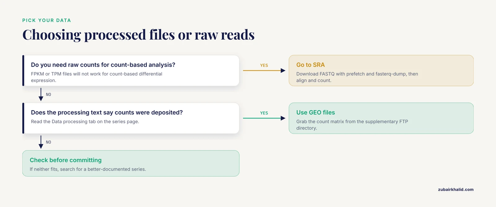
- Raw versus processed. Processed data means count matrices, FPKM or TPM tables, or cell-by-gene matrices deposited as supplementary files. Raw data means FASTQ files, which live in SRA. Decide early, because raw data requires an alignment and counting pipeline while processed data may only require careful quality checks.
- Design and replication. You need enough biological replicates per condition to support differential expression analysis. A well-described dataset states its design explicitly, for instance three biological replicates per genotype and treatment combination in a maize study [8], or 20 autism spectrum disorder samples versus 19 typically developing controls retrieved from GEO for a machine learning study [2].
- Library type. The library preparation matters for analysis. The maize dataset above used the QuantSeq 3' mRNA-Seq kit, which produces strand-specific reads targeted at the 3' end of transcripts [8]. A 3'-biased library behaves differently in alignment and quantification than a full-transcript library, so note the kit when you read the series page.
Write these five answers down as a one-line search specification before you touch the website. It becomes your query string.
How to Find RNA-Seq Datasets on NCBI GEO Step by Step
This walkthrough uses the GEO web interface at https://www.ncbi.nlm.nih.gov/geo/. Each step shows exactly what to click and what you should see.
Step 1. Open the GEO DataSets database and restrict to Series
From the GEO homepage, click Datasets, or go directly to https://www.ncbi.nlm.nih.gov/gds/. This search box queries the GEO DataSets index, which contains both Series (GSE records) and individual samples (GSM records). Left unfiltered, a keyword search returns a mix of both.
On the results page, look at the left sidebar under Entry type and select Series. This keeps only GSE records, which is what you want when hunting a whole experiment rather than one sample.
Step 2. Build a query with field tags
Type a query that combines your keywords with NCBI field tags. Useful tags in this database include [ORGN] for organism, [ETYP] for entry type, and [PDAT] for publication date. To find human single-cell RNA-seq datasets about keloids published since 2020, you would enter:
keloid[All Fields] AND gse[ETYP] AND homo sapiens[ORGN] AND 2020:2026[PDAT]If you already have an accession, skip the search entirely and paste it into the bar. Entering GSE176155 takes you straight to the kidney stone scRNA-seq series described earlier [5].
Step 3. Filter and scan the results list
Each result row shows the GSE accession, title, summary, organism, number of samples, platform, and whether supplementary files are available. Scan for three things:
- Sample count. A series with 6 samples can support a two-group comparison at best. A series with dozens of samples across multiple conditions offers more analytical room.
- Platform description. Look for high-throughput sequencing platforms rather than microarray platforms if you specifically want RNA-seq.
- Supplementary file availability. The icon column indicates whether processed or raw files are attached. A series with no supplementary files is often a dead end for reanalysis.
Step 4. Open the series page and read every tab
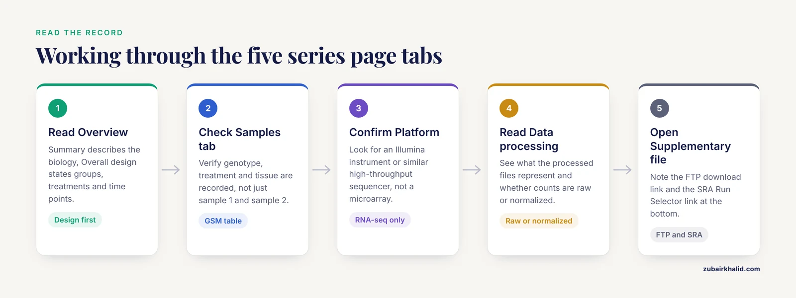
Click a GSE accession. A series page has five tabs, and each one answers a specific question:
- Overview. The Summary describes the biology. The Overall design states the experimental layout. Read both before anything else, because this is where submitters declare group structure, treatments, and time points.
- Samples. A table of every GSM with its title, source name, and characteristics. This is where you verify that the metadata you need, such as genotype, treatment, and tissue, was actually recorded. If the characteristics column says only "sample 1" and "sample 2," you will struggle to use this dataset.
- Platform. The sequencing instrument and assay. For RNA-seq you want to see an Illumina instrument or similar high-throughput sequencer.
- Data processing. The submitter's own pipeline description. This tells you what the processed files represent and what choices they made, which matters because different pipelines and normalization methods complicate comparison across studies [10].
- Supplementary file. The download links, discussed in the next section.
Step 5. Check the supplementary files and the SRA link
Scroll to the bottom of the Overview tab. You will typically see a line like:
Supplementary file     FTP download
                       SRA Run Selector
The FTP link gives processed files and bundled raw data if the submitter provided them. The SRA link takes you to the Run Selector, the grid view of all sequencing runs, from which raw FASTQ files are retrieved. A dataset descriptor for zebrafish exposed to uranyl nitrate and sodium arsenite, for example, deposited its raw data in GEO under accession GSE319292, and the counts and pathway statistics accompany the record [11].
Step 6. Record what you found
Before downloading anything, copy the GSE accession, the BioProject accession, the SRA study accession, the sample table, and the data processing text into a notes file. Two months from now, when a reviewer asks exactly which version you analyzed, this record is your only defense. A reusable analysis pipeline built on a documented accession trail is the difference between a reproducible project and a one-off [4].
Read the Series Page Before You Commit
Series pages vary enormously in quality, and a few minutes of reading prevents weeks of frustration. Work through this checklist:
Confirm the design matches your question. The Overall design field should state groups explicitly. If you plan a two-group differential expression comparison, confirm you have at least three biological replicates per group, which is the minimum most pipelines expect. Note that some datasets pool RNA before sequencing. In one bacterial dataset, RNA from three biological replicate cultures was pooled into a single sequencing library per strain and condition [6]. Pooled libraries reduce your effective sample size, and the dataset descriptor says so only if you read it.
Check the metadata depth. The Samples tab should let you reconstruct which file belongs to which condition. Datasets with rich characteristics fields, strain identifiers, and BioSample links (as in the bacterial example above [6]) are far easier to analyze than datasets where conditions are described only in the title.
Check for library kit quirks. QuantSeq 3' libraries produce reads concentrated at transcript 3' ends [8]. Standard gene-level count pipelines still work on them, but transcript-level quantification and splice-aware analyses do not. Similarly, small extracellular vesicle RNA or other specialized inputs behave unlike whole-cell RNA, so read the source description in the Samples tab.
Check the submitter's data processing text. If the series provides a counts matrix, the processing section should say how counts were generated and whether they are raw or normalized. Some series provide only FPKM or TPM values, which are suitable for some analyses but not for count-based differential expression methods that require raw counts.
For single-cell datasets, check what format the files are in. scRNA-seq reanalyses usually want raw cell-by-gene count matrices or the 10x Genomics matrix files, not just the processed cluster assignments. One keloid scRNA-seq reanalysis obtained data for eight patients from GEO and analyzed 73,790 cells, which was possible only because the deposited files supported full reprocessing [3]. Also expect large file sizes, often several gigabytes per sample.
Follow the cross-links. The series page links to PubMed (the associated paper, if any) and to SRA. A dataset descriptor paper, often published in the journal Data Brief, is a second source of documentation. The zebrafish toxicology dataset [11], the salicylic acid-treated tomato dataset with 12 SRA runs in three biological replicates [12], and the freshwater bacterial dataset [6] were all published as Data Brief articles precisely to document deposited data. Searching PubMed for Data Brief[Journal] AND your topic AND RNA-seq is a discovery method in its own right.
Mine the Literature for Accessions
Browsing GEO works when you know the keywords. The literature works when you know the question. Both routes converge on accessions, and published papers are the fastest way to find vetted, previously analyzed datasets.
Three patterns recur:
- Dataset descriptor papers. As above, Data Brief articles document deposited datasets and list accessions directly [11], [12], [6].
- Reanalysis papers. Integration and meta-analysis papers list every accession they used. The PDAC hub-gene study lists seven GEO accessions in one sentence [7]. A traumatic brain injury study states that its bulk and single-cell mouse datasets were retrieved from the NCBI GEO database [9]. An adenomyosis scRNA-seq study integrated its own data with the public normal endometrial series GSE183837 [13]. These papers have already done your first round of dataset screening.
- Methods and pipeline papers. Protocol papers demonstrate their pipelines on real data and name the accessions. A tuberculosis analysis demonstrated a custom annotation workflow on RNA-seq data from GSE292409, which captures the transcriptional response of Mycobacterium tuberculosis H37Rv to rifampicin [14]. Pipeline papers for Chlamydomonas reinhardtii name the SRA data they processed [10].
A practical habit: whenever you read an RNA-seq paper closely related to your project, search its methods section for strings matching GSE, SRP, SRR, or PRJNA and log them. Even papers you disagree with point you at the data.
Search GEO from the Command Line
The web interface is fine for one-off searches, but scripted discovery pays off when you want to track new datasets or screen hundreds of series. Two tools cover this.
Option A. E-utilities with any HTTP client
NCBI's E-utilities API works on the gds database, which indexes GEO. A basic search with curl:
curl "https://eutils.ncbi.nlm.nih.gov/entrez/eutils/esearch.fcgi?db=gds&term=GSE%5BETYP%5D+AND+sotorasib"Note that square brackets must be URL-encoded as %5B and %5D. The expected output looks like:
<eSearchResult>
  <Count>3</Count>
  <IdList>
    <Id>200xxxxxx</Id>
    ...
  </IdList>
</eSearchResult>
Series records carry UIDs in the 200-millions, and the GSE number is encoded in the UID. Fetch summaries for each UID to see titles, summaries, organism, and sample counts:
efetch -db gds -id 200xxxxxx -format docsumOption B. Entrez Direct (EDirect)
EDirect wraps E-utilities in Unix pipes. After installing it per NCBI's documentation:
esearch -db gds -query "GSE[ETYP] AND pancreatic ductal adenocarcinoma AND homo sapiens[ORGN]" \
  | efetch -format docsum \
  | grep -E "Accession|n_samples|title" \
  > pdac_candidates.txt
Each output block contains an <Accession> element (for example GSE136569), an <n_samples> element, and the title. Expected output looks like:
<Accession>GSE136569</Accession>
<n_samples>106</n_samples>
<title>High throughput sequencing of pancreatic ductal adenocarcinoma ...</title>
(Those specific numbers illustrate the format, check the live record for current values.) Filter on n_samples to drop datasets too small for your design, then open the shortlist in a browser and apply the series page checklist from the previous section.
Option C. From within R
The GEOquery Bioconductor package pulls series metadata and processed expression data directly into R:
library(GEOquery)
gse <- getGEO("GSE136569", GSEMatrix = TRUE)
gse <- gse[[14]]
dim(exprs(gse))
head(colnames(gse))
table(pData(gse)$characteristics_ch1)
Expected output for a typical series is a gene-by-sample expression matrix, with column names matching GSM accessions and the pData slot holding the sample characteristics. The RCPA package extends this idea with functions that download and process GEO data as the first step of a full pathway analysis workflow [15], which is convenient when your end goal is enrichment analysis rather than raw data handling.
Download the Data
What you download depends on whether you want processed matrices or raw reads.
Downloading processed files from GEO
Every series has a stable supplementary file directory on NCBI's FTP mirror, reachable over HTTPS. The directory path follows a fixed pattern: the third through fifth digits of the accession become an nnn folder. For GSE136569, the path is:
https://ftp.ncbi.nlm.nih.gov/geo/series/GSE136nnn/GSE136569/suppl/To fetch everything in that directory:
wget -r -np -nd -A "*RAW*" \
  https://ftp.ncbi.nlm.nih.gov/geo/series/GSE136nnn/GSE136569/suppl/
The flags mean: recurse (-r), do not ascend to parent directories (-np), do not recreate directory structure (-nd), and accept only files matching the pattern (-A). Expected output is a list of downloaded archives such as GSE136569_RAW.tar, which unpacks into per-sample count or matrix files, plus GSE136569_series_matrix.txt.gz, a plain-text file holding the full metadata table.
To fetch a single file instead:
wget https://ftp.ncbi.nlm.nih.gov/geo/series/GSE136nnn/GSE136569/suppl/GSE136569_series_matrix.txt.gzDownloading raw FASTQ files from SRA
GEO rarely hosts FASTQ files directly. Raw reads are retrieved from SRA with the SRA Toolkit, which is also the standard first step in published end-to-end protocols [4] and automated pipelines [10].
First, find the run accessions. From the series page, click the SRA Run Selector link, or note the SRR identifiers listed in a dataset descriptor such as the bacterial study with runs SRR38280322 through SRR38280329 [6]. Then:
prefetch SRR38280322
fasterq-dump SRR38280322 --split-files
gzip SRR38280322_1.fastq SRR38280322_2.fastq
prefetch downloads the run to a local cache and prints a progress line ending with the run accession. fasterq-dump extracts FASTQ files, and the -split-files option (two hyphens in the flag) keeps the mates of paired-end data in separate files, which is essential for paired-end alignment. Expected output for paired-end data is two files:
SRR38280322_1.fastq.gz
SRR38280322_2.fastq.gz
For a whole study, list the run accessions in a text file and loop:
cat SRR_Acc_List.txt | while read srr
do
  prefetch "$srr"
  fasterq-dump "$srr" --split-files
done
Key commands at a glance
| Task | Command or URL | Notes |
|---|---|---|
| Look up an accession | https://www.ncbi.nlm.nih.gov/geo/query/acc.cgi?acc=GSE136569 | Works for GSE and GSM |
| List supplementary files | .../geo/series/GSE136nnn/GSE136569/suppl/ in a browser | Pattern applies to any GSE |
| Grab all raw-bundled files | wget -r -np -nd -A "RAW" <suppl URL> | Single-dash flags only |
| Fetch one SRA run | prefetch SRR38280322 | Stores in local cache |
| Extract paired FASTQ | fasterq-dump SRR38280322, split-files | Two files for paired-end |
| Search GEO in a script | esearch -db gds -query "GSE[ETYP] AND <terms>" | Via EDirect or E-utilities |
| Pull a series into R | getGEO("GSE136569", GSEMatrix = TRUE) | GEOquery package |
Verify What You Downloaded
Downloads fail silently more often than you would like. Check three things before analysis:
File integrity. Compare file sizes against the sizes shown on the supplementary file page. If NCBI provides checksums, run md5sum <file> and compare. A truncated download of a multi-gigabyte 10x matrix is a classic cause of a parsing error an hour later.
Read structure. For FASTQ files, check that every record is four lines and that read names in the _1 and _2 files match in order:
zcat SRR38280322_1.fastq.gz | head -n 8
zcat SRR38280322_2.fastq.gz | head -n 8
The first and third lines of each record should begin with @SRR38280322 and + respectively, and the identifier portions of read names should align between the two mate files.
Biological sanity. Align a small subsample or inspect quality with FastQC, which is the standard first quality check in published workflows [4]. Alignment rates vary widely even within well-run datasets. The bacterial iron-limitation study reported alignment rates from roughly 35 percent to over 92 percent across its four strains [6], which is a useful reminder that a low alignment rate can reflect a genuine biological or reference-genome mismatch rather than a broken download. If your numbers look anomalous compared to the dataset descriptor, reread the descriptor before blaming your pipeline.
Practical Tips for Faster, Cleaner Searches
- Search by accession prefix, not keyword, whenever you have any accession at all. A paper mentioning PRJNA735197 takes you to BioProject, which links to the GEO series and every run [5].
- Use
[ETYP]and[ORGN]tags in every gds query. Unfiltered searches bury the series you want under thousands of individual sample records. - Sort or filter by sample count. Most differential expression work needs at least three replicates per group, so datasets with fewer than six samples rarely repay the download time.
- Prefer series with a linked publication. The paper documents the design, the analysis choices, and often the pitfalls, and reanalysis papers have already screened the dataset once [7], [9].
- Check the platform record for library details. Strandedness, single-end versus paired-end, and 3'-bias from kits like QuantSeq [8] all change the analysis pipeline you should use.
- Set up a repeatable query. Save your EDirect command in a script and rerun it monthly. New GEO series in your field will appear in the output, and the cost is one cron entry.
- For non-model organisms, check annotation status early. Functional enrichment for organisms like bacteria often requires building custom annotation resources from NCBI data before the expression analysis is even interpretable [14].
Common Mistakes and Limitations
Treating GEO and SRA as interchangeable. GEO holds processed files and metadata. FASTQ files are almost always in SRA, reached through the series page's SRA link. Downloading only the GEO supplementary files and then wondering where the reads are is the single most common beginner error.
Assuming every series has raw counts. Some submitters deposit only normalized values such as FPKM or TPM, or only a figures-ready matrix. Count-based differential expression methods need raw counts, so if the processing text does not say counts were deposited, plan to go to SRA and reprocess from reads.
Ignoring library preparation and strandedness. A 3'-tagged library such as QuantSeq [8] is not interchangeable with a full-transcript library in quantification, and unstranded treatment of stranded data inflates antisense artifacts. Check the platform and processing text.
Trusting sample titles instead of metadata. Titles like KM12C_rep1 may encode cell line and replicate but say nothing about treatment. The characteristics fields in the Samples tab and the BioSample records are the authoritative metadata [6].
Overlooking pooled samples. When RNA from three replicate cultures is pooled into one library, the deposited file count overstates the statistical replication [6]. Read the design description.
Downloading before checking scRNA-seq file formats. Single-cell reanalysis needs raw count matrices or 10x matrix bundles. If a series only provides processed cluster labels and marker tables, full reprocessing, as done in the keloid study with 73,790 cells [3], will not be possible.
Mixing data across platforms and pipelines without thought. Batch effects and differing normalization methods complicate cross-study comparison, a known challenge that motivates careful processing choices [10]. When pooling many GEO series, as in multi-dataset hub-gene screens, process each series consistently and model batch explicitly.
Forgetting that analysis results in the original paper may differ from yours. Different alignment and counting tools legitimately produce different count tables [10]. Your DEG list matching the original publication is a bonus, not a requirement, provided your pipeline is internally sound and documented.
Neglecting documentation of what you downloaded. Record accessions, download dates, file versions, and every filtering decision. End-to-end protocols emphasize reproducibility as a design goal, not an afterthought [4].
One structural limitation to plan around. Metadata quality in public repositories is uneven, and not every series records everything you need. When a dataset's metadata cannot answer your question, the correct move is to search for a better-documented series rather than to guess labels from file names.
Frequently Asked Questions
Is GEO data free to download?
Yes. All GEO data, including supplementary files and series matrices, are publicly available without registration, and raw reads in the linked SRA records are free as well.
What is the difference between GEO and SRA?
GEO stores expression matrices, sample metadata, and experiment descriptions, while SRA stores the raw sequencing reads in FASTQ format. A GEO series page links to its corresponding SRA records for raw data access.
What is a GSE accession?
A GSE accession identifies a GEO Series, meaning one complete experiment with its samples, platform, metadata, and supplementary files. It is the standard unit researchers cite and download.
Can I find single-cell RNA-seq datasets on GEO?
Yes. GEO hosts a large and growing collection of single-cell RNA-seq series alongside bulk RNA-seq, and many published reanalyses start from public scRNA-seq accessions.
How do I download FASTQ files from a GEO series?
Open the series page, follow the SRA Run Selector link, note the SRR run accessions, then run prefetch and fasterq-dump from the SRA Toolkit on each run.
How do I search GEO from the command line?
Use NCBI E-utilities or Entrez Direct against the gds database, filtering on the GSE entry type, or use the GEOquery and RCPA R packages to retrieve series programmatically.
How do I know if a dataset has enough replicates?
Read the Overall design field and the Samples tab on the series page, counting independent biological samples per condition, and watch for pooled libraries that reduce true replication.
How do I cite a GEO dataset in a paper?
Cite the GSE accession together with the associated publication if one exists, and give the accession and download date in your methods section so others can retrieve the identical data.
Sources
- Potential biomarkers uncovered by bioinformatics analysis in sotorasib resistant-pancreatic ductal adenocarcinoma.
- Identification of Potential Biomarkers in ASD Integrating RNA Seq Data and Machine Learning Approaches.
- Integrated multi-omics analysis reveals key molecular mechanisms underlying fibroproliferation and immune dysregulation in keloids.
- Streamline Protocol for Bulk-RNA Sequencing: From Data Extraction to Expression Analysis.
- Expression analysis of epithelial membrane protein 1 (EMP1) gene in kidney stone patients.
- Transcriptome datasets of four freshwater bacterial isolates grown under iron-replete and iron-limited conditions.
- Dysregulated expression of cell cycle regulators CDC20, PLK1, BUB1, CDC45, CDCA5 in pancreatic ductal adenocarcinoma.
- Illumina RNA-seq data of Genotype-specific responses of maize plants to Funneliformis mosseae.
- Decoding microglial metabolic cell death and PANoptosis hub genes in subacute phase of traumatic brain injury: a multi-omics and experimental validation study.
- Development and validation of the PipeSeq program for RNA-seq data analysis in the Chlamydomonas reinhardtii as a model.
- Transcriptomic data of larval zebrafish exposed to environmentally relevant levels of uranyl nitrate and sodium arsenite.
- Transcriptome datasets of salicylic acid-treated tomato plant cultures under normal and stress conditions.
- FSP1+ stromal cell-associated macrophage efferocytosis contributes to impaired decidualization in adenomyosis.
- Enhanced RNA-Seq Expression Profiling and Functional Enrichment in Non-model Organisms Using Custom Annotations.
- RCPA: An Open-Source R Package for Data Processing, Differential Analysis, Consensus Pathway Analysis, and Visualization.