How to Make a Publication-Ready Heatmap in R for Gene Expression Data
By Dr. Zubair Khalid, DVM, MS, PhD ·

By the end of this guide you will be able to take a raw gene expression matrix, select the genes worth showing, cluster and annotate them, and export a heatmap that survives peer review at journal resolution. You need a current R installation, roughly an hour of focused work, and the packages listed below. Everything runs in plain R scripts, so every figure regenerates from code with one command.
The heatmap is one of the most reproduced figure types in gene expression publishing. Recent papers use it to show salinity-responsive genes sorting into distinct expression patterns across time points in tomato [1], to display tissue- and age-specific expression of a 44-member transcription factor family in ginseng [2], to compare shared upregulated genes between pancreatic cancer and diabetes datasets mined from GEO [3], to visualize diel clock gene expression measured in water samples versus fish tissues [4], and to display inflammatory protein abundance patterns in tear fluid proteomics [5]. The pattern is consistent. A heatmap works when it summarizes a result that statistics already established, and it fails when it tries to carry the argument by itself.
Why Gene Expression Heatmaps Earn Their Place in a Published Figure
A heatmap displays a matrix of values as a color grid, usually with hierarchical clustering dendrograms on the rows and columns. In gene expression work it answers one visual question quickly: which genes behave the same way across which samples.
Published papers use the figure in three distinct roles, and knowing which role yours plays determines every downstream choice.
First, the descriptive role. Gene family papers routinely organize expression heatmaps by tissue, developmental stage, or species, showing that members have specific expression patterns rather than uniform behavior [2]. Sugarcane HCT gene family work took the same idea further and connected subgroup-level expression patterns to regulatory elements in the promoters [6]. In these figures the grouping often comes from biology you already know, such as phylogenetic subgroups, rather than from clustering the data.
Second, the pattern-discovery role. In the tomato salinity study, hierarchical clustering and heatmap analyses demonstrated distinct expression patterns among genes across different salinity levels and sampling times [1]. In the environmental RNA study of grouper clock genes, heatmap visualization supported the conclusion that signals from rearing water tracked tissue expression over the day [4]. Here the clustering itself is part of the message.
Third, the exploratory-support role. The isoserine study in APP/PS1 mice profiled 84 synaptic-related genes on a targeted PCR array, used exploratory heatmaps and principal component analysis to illustrate disease-context-dependent expression patterns, and paired those figures with module-level tests that reached FDR significance even though individual gene-level effects did not survive correction [7]. That pairing is the textbook pattern for a well-behaved heatmap. The figure illustrates. The statistics decide.
What Publication-Ready Actually Means
A publication-ready heatmap satisfies five concrete requirements.
- The data are transformed appropriately, meaning normalized expression values, not raw counts, and usually row-standardized so color reflects relative pattern rather than absolute abundance.
- Clustering choices are deliberate and reportable. You know the distance metric, the linkage method, and whether the column order reflects clustering or experimental design.
- Annotations identify samples and genes so a reader can interpret the pattern without reading your methods in detail.
- The color scale is perceptually even, colorblind-safe, and has explicit limits that match the data.
- The figure exports at the resolution and dimensions the journal specifies, typically 300 dpi or higher for raster files or a vector format such as PDF.
Anything less produces a figure that reviewers flag and that you regenerate three times. The steps below get you there in one pass.
Installing the Toolkit: R for Bioinformatics Basics
R for bioinformatics divides its packages between CRAN, the general R archive, and Bioconductor, the project that curates genomic packages with standardized data classes and tutorial-style vignettes. Every Bioconductor package ships with a vignette that functions as a runnable Bioconductor tutorial, and reading the vignette for DESeq2 or limma before using them is the fastest way to avoid analysis errors.
# Install Bioconductor's package manager if it is not present
if (!requireNamespace("BiocManager", quietly = TRUE)) {
  install.packages("BiocManager")
}

# Bioconductor packages for data acquisition, testing, and heatmaps
BiocManager::install(c("GEOquery", "limma", "DESeq2", "ComplexHeatmap"))

# CRAN packages for basic heatmaps and color control
install.packages(c("pheatmap", "dplyr", "RColorBrewer", "viridis"))
You need four of these for the core workflow. GEOquery downloads data from the Gene Expression Omnibus, the NCBI public repository of expression data. limma and DESeq2 perform differential expression testing for microarray and RNA-seq data respectively. pheatmap and ComplexHeatmap draw the figures. For interactive exploration before you commit to a static figure, dedicated Shiny applications built on DESeq2 combine heatmaps, PCA, and correlation views in one interface, which is exactly how modern poultry genomics tools such as INFO GRAB are structured [8], and web resources such as the eQTM Atlas expose gene expression associations through built-in heatmap interfaces for the same reason [9].
Heatmap in R for Gene Expression, Step by Step

The walkthrough uses a real dataset so every command does something observable. The diabetic retinopathy series GSE102485 contains 3 normal control and 22 diabetic retinopathy samples and was analyzed with limma in its original publication [10]. Any expression matrix in a data frame or matrix object works with identical commands.
Step 1. Pull a Gene Expression Matrix from GEO
library(GEOquery)

# Download the series matrix. This fetches the processed expression values,
# not raw sequencing files.
gse <- getGEO("GSE102485", GSEMatrix = TRUE)[[7]]

expr <- exprs(gse)
dim(expr)   # rows = one per probe or gene, columns = one per sample
GEOquery prints download and parsing messages to the console and returns an ExpressionSet. The exprs() accessor extracts the numeric matrix. Check the shape immediately with dim() and check the value distribution with summary(as.vector(expr)). If the series stores raw counts instead of processed values, the summary shows very large integers and you should switch to the RNA-seq path in Step 3.
For a comparative design like the pancreatic cancer and diabetes integration study, you would repeat this step for each accession, here GSE15471 and GSE20966, harmonize gene identifiers, and then intersect the differential expression results before plotting shared upregulated genes [3].
Step 2. Clean and Transform the Matrix
Publication heatmaps almost always display log-scale or standardized values. Log2 transformation makes fold changes symmetric, so a fourfold increase reads as +2 and a fourfold decrease reads as -2.
# Log2 transform if the data are not already on the log scale.
# Log-transformed microarray values typically span a small range such as 2 to 14.
if (max(expr) > 100) {
  expr_log <- log2(expr + 1)
} else {
  expr_log <- expr
}

# Remove rows with missing values, which break clustering later.
expr_log <- na.omit(expr_log)

# Remove rows with near-zero variance, which carry no pattern to show.
sd_vec <- apply(expr_log, 1, sd)
expr_log <- expr_log[sd_vec > 1e-8, ]
The variance filter matters more than it looks. Zero-variance genes produce NA values under correlation-based distances and crash the clustering step with an obscure error. Filtering them now prevents that failure entirely.
Step 3. Choose the Genes to Display
There are two defensible selection strategies. For a hypothesis-driven figure, test differential expression and show the significant genes. For a survey figure, show the most variable genes.
The statistical route, using limma for microarray data as in the original analysis of this dataset [10]:
library(limma)

# Build the group factor from sample metadata. Inspect the column names
# first because GEO annotation names vary by series.
colnames(pData(gse))
group <- pData(gse)$characteristics_ch1   # adjust to the actual column
group <- factor(grepl("diabetic|DR", group, ignore.case = TRUE),
                labels = c("Control", "DR"))

design <- model.matrix(~ 0 + group)
colnames(design) <- levels(group)
fit  <- lmFit(expr_log, design)
contr <- makeContrasts(DR - Control, levels = design)
fit2 <- eBayes(contrasts.fit(fit, contr))
res  <- topTable(fit2, number = Inf, adjust.method = "BH")

# Differentially expressed genes: FDR below 0.05 and absolute log2
# fold change above 1 (a twofold change).
deg <- subset(res, adj.P.Val < 0.05 & abs(logFC) > 1)
False discovery rate, or FDR, corrects p-values for the thousands of simultaneous tests in a gene expression experiment. Benjamini-Hochberg adjustment is the standard default and is what adjust.method = "BH" invokes.
Then select the genes for the figure. Fifty to two hundred genes is the range where a printed heatmap stays legible with visible row labels:
# Top 50 by absolute log2 fold change, mixing up and down regulation
top_ids <- head(order(-abs(res$logFC)), 50)

mat <- expr_log[top_ids, ]
For the survey route on RNA-seq count data, use DESeq2, apply the variance stabilizing transform, and take the most variable genes:
library(DESeq2)
dds <- DESeqDataSetFromMatrix(countData = round(expr_raw),
                              colData   = coldata,
                              design    = ~ group)
dds <- DESeq(dds)
vsd <- vst(dds, blind = FALSE)

rv    <- apply(assay(vsd), 1, var)
top_g <- names(head(sort(rv, decreasing = TRUE), 500))
mat   <- assay(vsd)[top_g, ]
vst() converts counts to a scale where the variance no longer depends on the mean, which is a prerequisite for honest clustering of RNA-seq data.
Step 4. Draw a First Heatmap with pheatmap
pheatmap produces a clustered, annotated heatmap in one call and is the fastest path from matrix to draft figure.
library(pheatmap)

# Row-standardize: convert each gene's values to z-scores so the color
# encodes the pattern, not the abundance.
mat_z <- t(scale(t(mat)))

pheatmap(mat_z,
         scale = "none",           # already scaled manually
         clustering_method = "ward.D2",
         border_color = NA,
         fontsize_row = 6)
The t(scale(t(mat))) idiom is worth memorizing. scale() standardizes columns of a matrix. Transposing first puts genes in columns, so scaling computes each gene's mean and standard deviation across samples. The z-score is the number of standard deviations a value sits from its row mean. A red cell then means "this gene is high in this sample relative to its average behavior," which is usually the biological question.
pheatmap prints nothing to the console and draws to the current plotting device. On the first run you should see a square-ish grid, two dendrograms, a color legend on the right, and row labels that are probably unreadable probe IDs. Unreadable labels are the next problem to fix.
Step 5. Add Sample Annotations
Annotations are the colored side bars that map each column to a condition. They turn a decorative figure into an interpretable one.
# One row per sample, one column per annotation. Row names must match
# colnames(mat) exactly.
coldata <- data.frame(Group = group,
                      row.names = colnames(mat))

ann_colors <- list(
  Group = c(Control = "grey85", DR = "#b2182b")
)

pheatmap(mat_z,
         scale = "none",
         annotation_col = coldata,
         annotation_colors = ann_colors,
         clustering_method = "ward.D2",
         border_color = NA,
         fontsize_row = 7,
         main = "Top 50 differentially expressed genes (GSE102485)")
If you map gene identifiers to symbols before plotting, do it with a proper annotation mapping rather than string matching, and collapse duplicate symbols by keeping the row with the highest mean or variance. Probe-level heatmaps with dozens of rows for the same gene read as noise to reviewers.
Step 6. Take Control of the Clustering
Two parameters define the entire tree structure, and defaults are not always what you want.
Distance metric. Euclidean distance on z-scored rows and Pearson correlation distance ("correlation" in pheatmap) usually agree after standardization. Correlation distance has one advantage that matters in practice: it groups genes by pattern shape even when their z-score magnitudes differ. On unscaled data, it is the safer choice.
Linkage method. Ward linkage ("ward.D2" in R) produces compact, similarly sized clusters and has become the de facto standard in gene expression figures. Complete linkage produces tighter chains. Single linkage produces the long stringy trees that reviewers dislike.
pheatmap(mat_z,
         clustering_distance_rows = "correlation",
         clustering_method = "ward.D2",
         cutree_rows = 4,          # cut the row tree into 4 modules
         annotation_col = coldata,
         annotation_colors = ann_colors,
         border_color = NA)
cutree_rows slices the dendrogram at a height that yields the requested number of clusters and draws white separator lines between them. Choose the number by looking at the dendrogram, not by trial and error on the final figure.
A deliberate alternative to clustering columns is imposing the sample order that reflects your design, for example time points in increasing order. The tomato salinity study benefited from exactly this logic because its columns were defined salinity levels and day 15 versus day 45 sampling times [1], and the grouper clock gene analysis likewise compared defined time points rather than clustered samples [4]. When column order carries experimental meaning, set cluster_cols = FALSE in pheatmap and order the matrix yourself.
Step 7. Refine Color, Text, and Geometry
The default red-yellow palette is not colorblind safe. Two palettes cover almost every publication need:
# Diverging palette for z-scored data, centered on white
pal_div <- colorRampPalette(c("#2166ac", "white", "#b2182b"))(100)

# Sequential palette for non-negative values such as TPM or percent
pal_seq <- colorRampPalette(c("#f7f7f7", "#4393c3", "#053061"))(100)
Because z-scores are symmetric around zero, the color scale should be too. Set symmetric limits so white means neutral:
lim <- max(abs(mat_z))
pheatmap(mat_z,
         color = pal_div,
         legend_breaks = seq(-ceiling(lim), ceiling(lim), by = 2),
         annotation_col = coldata,
         annotation_colors = ann_colors,
         border_color = NA,
         fontsize_row = 7,
         fontsize_col = 9,
         cellwidth = 12,
         cellheight = 11)
cellwidth and cellheight are in points and control the physical figure size. For a 50 gene by 25 sample heatmap, the values above give roughly a 300 by 550 point figure. Small cells with border_color = NA read cleanly, while borders on small cells turn the figure into a grid of gray lines.
Step 8. Build Multi-Panel Figures with ComplexHeatmap
When a single grid is not enough, for example when you want to attach a dot plot of fold changes, a bar of pathway membership, or several matrices stacked vertically, move to ComplexHeatmap. The package is the Bioconductor standard for composable heatmap figures, and the recent ggalign package extends the same idea within the ggplot2 grammar of graphics, with a dedicated protocol for gene expression matrix heatmaps among its published set of visualization protocols [11].
library(ComplexHeatmap)
library(circlize)

col_fun <- colorRamp2(c(-2, 0, 2),
                      c("#2166ac", "white", "#b2182b"))

ha <- HeatmapAnnotation(
  Group  = coldata$Group,
  col    = list(Group = c("Control" = "grey85", "DR" = "#b2182b")),
  annotation_name_gp = gpar(fontsize = 9)
)

set.seed(42)
ht <- Heatmap(mat_z,
              name = "z-score",
              col = col_fun,
              top_annotation = ha,
              clustering_method_columns = "ward.D2",
              clustering_distance_rows = "correlation",
              row_km = 4,
              row_names_gp = gpar(fontsize = 7),
              column_names_gp = gpar(fontsize = 8),
              rect_gp = gpar(col = NA),
              column_title = "Diabetic retinopathy vs control",
              heatmap_legend_param = list(title = "z-score"))
ht
row_km = 4 replaces pheatmap's cutree_rows with k-means partitioning of the rows. K-means starts from random positions, so set.seed() before the call is what makes the figure reproducible between runs. column_split = coldata$Group is the companion argument when you want columns pre-divided by condition before clustering within each block.
A useful trick for time-course or dose-response data is to plot each time point as its own heatmap component in the same figure and let ComplexHeatmap align the row order across components. That design directly mirrors the published salinity analysis structure, where gene patterns separated by both stress intensity and sampling day [1].
Step 9. Export at Journal Resolution
Most journals ask for 300 dpi at final print size for raster images, or a vector PDF or SVG. Raster formats are pixel grids, vector formats are mathematical descriptions that scale without loss. For a heatmap, vector output is preferable whenever the file size stays reasonable.
# pheatmap writes directly to file with the filename argument
pheatmap(mat_z,
         color = pal_div,
         annotation_col = coldata,
         annotation_colors = ann_colors,
         filename = "heatmap_gse102485.pdf",
         width = 7, height = 9)

# ComplexHeatmap requires an explicit device
pdf("heatmap_gse102485.pdf", width = 7, height = 9)
draw(ht)
dev.off()

# Raster alternative at journal resolution
png("heatmap_gse102485.png", width = 7, height = 9,
    units = "in", res = 300)
draw(ht)
dev.off()
Always set width, height, and units together. The classic failure, Error in plot.new() : figure margins too large, means the device is smaller than the content. Enlarge width or height rather than shrinking fonts. Never use JPEG for a heatmap, because its lossy compression smears the flat color blocks into visible artifacts around text.
Step 10. Sanity-Check the Figure
Four checks take two minutes and catch most errors before a reviewer does.
- Compare against PCA. Run
prcomp(t(mat_z))and plot the first two components colored by group. If PCA separates the groups and the heatmap does not, or vice versa, something is wrong in one of the two calculations. The pairing of PCA and heatmap as complementary checks appears across published workflows, including the tear proteomics study that used both to reveal abundance patterns between healthy and disease groups [5]. - Verify the color legend. The minimum and maximum on the color bar should roughly match the range of
mat_z, and white should sit at zero for z-scored data. - Confirm sample identity. Cross-reference a few column names against the metadata. Mislabeled columns are the single most damaging silent error in expression figures.
- Check the direction of the color mapping. With the blue-white-red palette above, blue means below the row mean and red means above. State this in the figure legend explicitly, because a reviewer should never have to guess.
Key Parameters at a Glance
| What you control | pheatmap argument | ComplexHeatmap argument | Effect |
|---|---|---|---|
| Row standardization | scale = "row" | scale = "row" in Heatmap() | Converts each gene to z-scores so color shows pattern, not abundance |
| Row distance | clustering_distance_rows | same name | Metric used to compare genes, "correlation" or "euclidean" |
| Linkage method | clustering_method | same name | Tree-building rule, "ward.D2" gives compact clusters |
| Split rows into modules | cutree_rows | row_km | Cuts the dendrogram or runs k-means, needs set.seed() in the k-means case |
| Column splitting | cluster_cols, manual ordering | column_split | Impose design order or pre-divide samples by condition |
| Sample annotations | annotation_col, annotation_colors | HeatmapAnnotation() in top_annotation | Colored bars that map samples to conditions |
| Color mapping | color, legend_breaks | col = colorRamp2(...), heatmap_legend_param | Palette and explicit scale limits |
| Cell size | cellwidth, cellheight | width, height per component | Physical dimensions in points |
| Cell borders | border_color = NA | rect_gp = gpar(col = NA) | Removes grid lines so dense matrices read cleanly |
| Direct file output | filename, width, height | explicit pdf() or png() device | Controls export resolution and format |
Heatmap Tips That Reviewers Notice
Annotate by biology, not by availability. A column annotation bar for treatment group, genotype, or time point earns its space. A bar for batch identifiers belongs there too if batch effects could explain part of the pattern, because showing them signals that you understood the confounding rather than hid it.
Match the clustering to the question. If the paper's argument is about predefined subgroups, as in gene family papers where phylogenetic subfamilies structure the figure [2] [6], impose that order rather than clustering rows. Clustering can separate a subfamily into two branches and visually contradict the phylogenetic figure above it, which invites reviewer confusion.
Pair the heatmap with a statistical test at the right level. The isoserine study is a useful template because it drew exploratory heatmaps but anchored its claims on module-level FDR-significant results after gene-level effects failed correction [7]. A heatmap of nominal findings with no corrected test is a figure that a methods reviewer will treat as decoration.
Use interactive tools during analysis, static figures for the paper. Shiny applications let you toggle genes, scales, and annotations quickly without rerunning scripts, which is why dedicated expression browsers build heatmaps and PCA into the same interface [8]. The final figure should still regenerate from a plain script for reproducibility.
Limit the legend vocabulary. Every distinct color in the annotation bars needs a meaning a reader can recall. More than five annotation colors per bar and the figure stops communicating. Consolidate categories before plotting.
State the preprocessing in the figure legend or methods. One sentence covers it: values are variance-stabilized and row z-score standardized, hierarchical clustering uses Ward linkage on correlation distance, and the color scale spans the symmetric range shown. Reviewers look for exactly this sentence.
Common Mistakes and Limitations
Heatmapping raw counts. Raw RNA-seq counts confound each gene's display range with library size and mean-variance structure. Normalize first with vst() in DESeq2 or log2 transformation after a scaling normalization in limma. A heatmap of raw counts can look striking and mean almost nothing.
Skipping row standardization. Without scale = "row", the two highest-abundance genes determine the entire color range and the other 98 genes render as near-white noise. The symptom is a figure where one or two rows glow and everything else looks flat. The fix is the t(scale(t(mat))) idiom from Step 4.
Zero-variance genes crashing the cluster step. With correlation distance, a gene with identical values across all samples yields a correlation of NA, and clustering fails with an error ending in NA/NaN/Inf in foreign function call (arg 1). The variance filter in Step 2 prevents this. If you see the error on an existing script, run any(apply(mat, 1, sd) == 0) to find the culprit rows.
Annotation and matrix name mismatches. annotation_col rows must match colnames(mat) exactly, including whitespace. A silent mismatch produces either an error about annotation dimensions or annotation bars full of NA. Guard against it with stopifnot(identical(rownames(coldata), colnames(mat))) before every plotting call.
Showing too many genes. A heatmap of 2,000 genes with row labels is a texture, not a figure. Either aggregate to module-level summaries, show a curated gene set, or show the top 50 to 100 features and reference a supplement for the full matrix. Reviewers consistently prefer the curated version.
Treating the heatmap as evidence. Clustering is descriptive. It cannot tell you whether a treatment effect is significant, and dendrogram branches have no p-values in standard implementations. Every inferential claim needs a test with correction for multiple comparisons, as the PCR array study demonstrated when its module-level tests carried claims that individual gene tests could not [7].
Non-reproducible clustering. K-means-based row splitting in ComplexHeatmap changes between runs unless you call set.seed() first. If a coauthor gets a different figure from your script, this is the usual cause.
Export problems. Low-resolution PNG exports turn tick labels into mush, and the figure margins too large error means the device size does not fit the content. Export at the final intended physical size rather than drawing large and scaling down in the manuscript.
The broader limitation is honest and worth stating plainly. A heatmap is a summary display. It compresses thousands of measurements into a color grid, and compression always discards information, so any biological conclusion needs support from the underlying statistics, replication, or validation experiments. The heatmap earns its place as the figure that lets a reader grasp the organized result, not as the analysis that produced it.
Frequently Asked Questions
What does scale = "row" actually do?
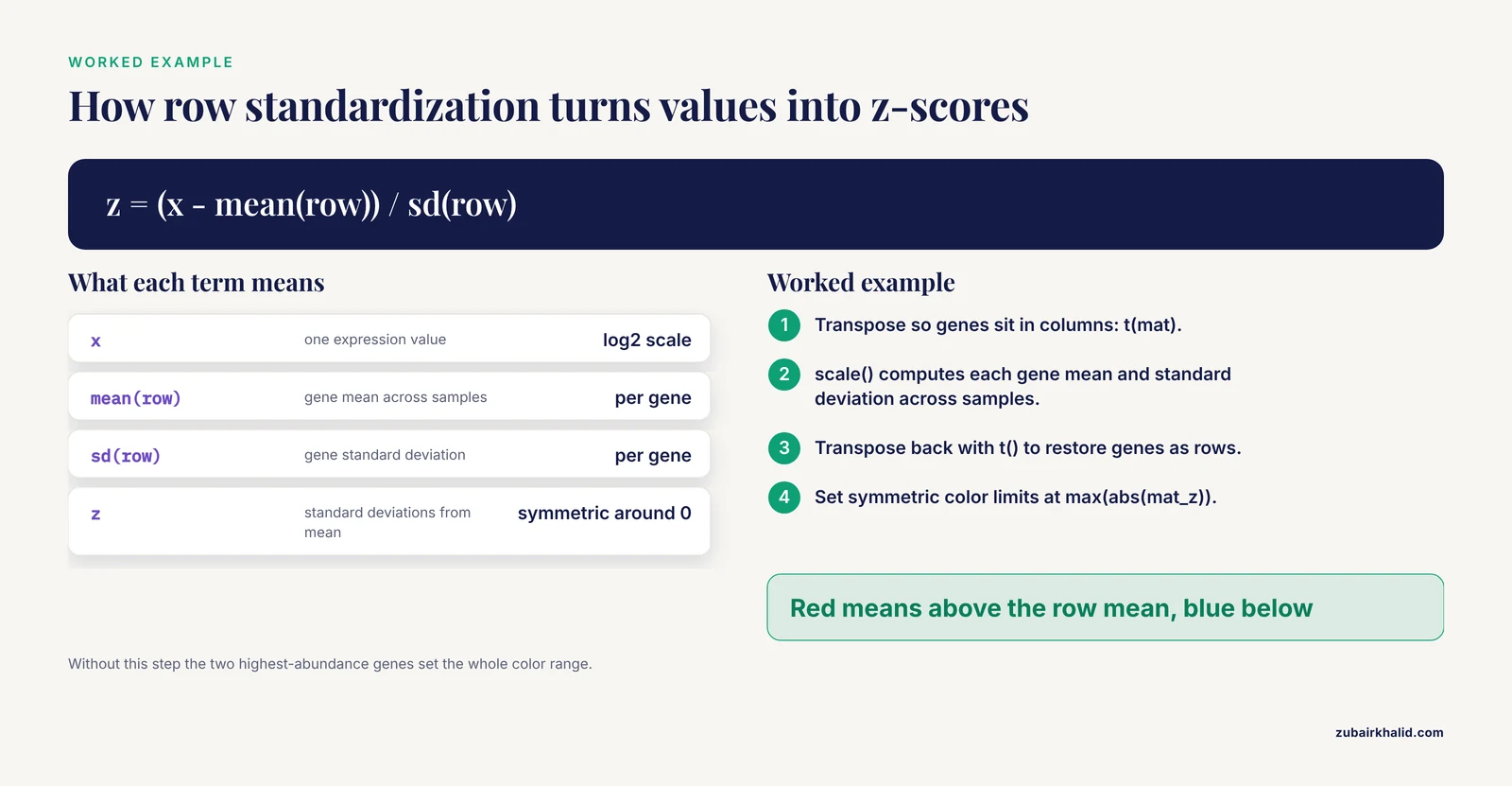
It converts each gene's values to z-scores, which are the number of standard deviations each value sits from that gene's mean across samples. This makes color reflect the relative pattern of each gene rather than its absolute expression level, and it is the right default for most gene expression heatmaps.
How many genes should I show in a heatmap?
Between roughly 50 and 200 if you want readable row labels, or a few hundred if you drop individual labels and rely on cluster labels. Beyond that, split the figure into modules or move the full matrix to a supplement.
Should I cluster both rows and columns or impose sample order?
Cluster rows when you want to discover gene modules. Impose column order when the sample order carries meaning, such as time points or dose levels, by setting cluster_cols = FALSE and arranging the matrix by your design.
Which color palette should I use?
For z-scored data, a diverging blue-white-red palette with symmetric limits. For non-negative values such as abundance, a sequential palette. Palettes from the viridis and RColorBrewer packages are colorblind-safe and widely accepted by journals.
Should I use pheatmap, ComplexHeatmap, or ggplot2?
Use pheatmap for a single clustered annotated heatmap, ComplexHeatmap when you need multi-panel compositions with attached annotations, and ggplot2-based tools such as ggalign when your whole figure pipeline lives in the ggplot2 grammar of graphics.
Do I need FDR-corrected p-values before drawing a heatmap?
You need them before making inferential claims about the genes shown. A heatmap can display exploratory patterns, but any statement that genes differ between conditions requires testing with multiple-comparison correction.
How do I save the heatmap at 300 dpi?
Call png() with width, height, units = "in", and res = 300 before drawing, or pass filename plus width and height directly to pheatmap. For vector output, use pdf() instead.
Can I use the heatmap itself as statistical evidence?
No. A heatmap is descriptive and its dendrograms carry no significance values. Use it to illustrate results established by differential expression testing, module-level analysis, or other inferential methods.
Sources
- Integrated physiological, biochemical, and gene expression responses of tomato (Solanum lycopersicum L.) to time-dependent salinity stress.
- Comprehensive Identification of CPP Gene Family Members in Panax ginseng and Expression Analysis of PgCPP and Key Protopanaxadiol Ginsenoside Biosynthesis Genes in Response to MeJA.
- Epidemiological Trends and Shared Molecular Signatures of Pancreatic Ductal Adenocarcinoma and Diabetes: An Integrative Analysis Based on Global Burden of Disease and Gene Expression Omnibus Datasets.
- Polyester wool-based environmental RNA collection enables detection of diel per2 expression in the Malabar grouper (Epinephelus malabaricus).
- Association of IL-8 and IL-18 Expression With Histone-Associated NETosis in Aqueous-Deficient and Evaporative Dry Eye Disease.
- Genome-wide identification of HCT gene family in sugarcane (Saccharum spp. hybrid) and characterization of putative cis-elements in gene regulation.
- Isoserine Improves Spatial Memory and Remodels Synaptic and Inflammatory Gene-Expression Programs in APP/PS1 Mice.
- INFO GRAB: An interactive shiny application for gene expression analysis and visualization.
- eQTM (expression quantitative trait methylation) Atlas: a comprehensive resource of over 11 million DNA methylation-gene expression associations through across 11 tissues and 4 diseases.
- Correlation between the expression levels of miR-199a-3p and FN1 in serum and aqueous humor and the severity of type 2 diabetic retinopathy in a Chinese population.
- Composable Visualization of High-Dimensional Biological Data with ggalign.