How to Create Custom Genome Browser Tracks in R with Gviz

By Dr. Zubair Khalid, DVM, MS, PhD · 2026-11-11

By the end of this article you will be able to build a publication-quality genome browser figure in R: an axis, a chromosome ideogram, a gene model, your own annotation intervals, a quantitative signal track from a bigWig file, a variant track from a VCF, and a nucleotide sequence track, all rendered in a single call to plotTracks(). You will also know how to fix the errors that stop most people on their first attempt.

To follow along you need R (4.1 or newer works well), the Bioconductor packages Gviz, GenomicRanges, rtracklayer, GenomeInfoDb, AnnotationHub, ensembldb, and VariantAnnotation, and optionally a BAM, bigWig, GTF, FASTA, or VCF file from your own project. Everything is free and runs on Windows, macOS, and Linux.

Why Gviz belongs in your r-for-bioinformatics toolkit

A genome browser view answers a question that tables of coordinates cannot: what does this locus look like, and what overlaps what? Gviz is a Bioconductor package built around this exact task. It takes genomic intervals and quantitative data, arranges them as stacked horizontal tracks, and draws a figure that reads like a snapshot of a browser session, except that every element is scripted and reproducible.

The need for this kind of contextual visualization is well recognized. The yEvo Mutation Browser, a web tool built in R Shiny to help students and researchers interpret whole-genome sequencing of experimentally evolved yeast, centers on a chromosome map of mutated genes and a gene viewer that places mutation sites inside their genomic and protein context [1]. The motivation is the same whether the audience is a classroom or a journal reviewer: a variant or a peak only makes sense against the gene model, the neighboring features, and the sequence around it. Gviz gives you that context as a scriptable, static figure.

Static scripted figures and interactive browsers solve different problems. Interactive tools such as IGV are ideal for exploratory clicking. Gviz excels when you need the same locus rendered for ten samples, or the same figure regenerated when the annotation release changes, or a figure embedded in an automated report. R is well suited to this pattern because it combines analysis and figure generation in one script, a strength that tutorial authors across quantitative disciplines keep demonstrating with fully scripted, command-by-command examples [2]. The Bioconductor ecosystem, where packages ship with documented data classes and vignettes, reinforces this scripted style.

Installing Gviz and the supporting packages

Install from Bioconductor, not CRAN. Gviz is distributed only through Bioconductor.

if (!require("BiocManager", quietly = TRUE))
    install.packages("BiocManager")

BiocManager::install(c("Gviz", "GenomicRanges", "rtracklayer",
                       "GenomeInfoDb", "AnnotationHub",
                       "ensembldb", "VariantAnnotation"))

Verify the installation and record your versions, which you will need for reproducibility later.

packageVersion("Gviz")        # for example, 3.20.x, depending on your release
sessionInfo()                 # capture the full package set for your report

If BiocManager reports that packages need updating, let it. Gviz depends on several core Bioconductor classes, and mixed versions of GenomicRanges and rtracklayer are a frequent source of confusing errors.

How Gviz thinks: tracks, ranges, and plotTracks

Three concepts carry the whole package.

First, a track is an object holding one layer of the figure. Each track class has a name: GenomeAxisTrack draws a ruler, IdeogramTrack draws the chromosome with its cytoband staining pattern, AnnotationTrack draws intervals, GeneRegionTrack draws transcripts with exons and UTRs, DataTrack draws numeric signal, and SequenceTrack draws nucleotides.

Second, the raw geometry lives in a GRanges object, the standard Bioconductor container for genomic intervals with chromosome, start, end, strand, and metadata columns. Every interval-based track either wraps a GRanges you supply or builds one internally from a database.

Third, plotTracks() is the single renderer. It takes a list of track objects plus a genomic window and draws them top to bottom in the order you list them. Almost all cosmetic control happens through displayPars, a named list of parameters attached to each track.

This separation matters because it means you prepare data with ordinary GRanges operations (subsetting, subsetByOverlaps, resize, findOverlaps) and only think about appearance at the last step.

A step-by-step walkthrough: a publication-ready locus figure

This g-viz tutorial in R step by step section builds one figure around the human TP53 locus on chromosome 17 using GRCh38 (UCSC identifier hg38). Substitute your own chromosome and coordinates; the structure of the code does not change.

Step 1: load packages and define the plotting window

library(Gviz)
library(GenomicRanges)
library(rtracklayer)

chr    <- "chr17"
region <- GRanges("chr17", IRanges(7668421, 7687489))  # TP53 body, hg38

Always define the window as a GRanges early. You will reuse it to subset annotation, to restrict file imports, and as the from/to arguments of plotTracks(), which keeps every layer consistent.

Step 2: the axis and the ideogram

atr <- GenomeAxisTrack()
itr <- IdeogramTrack(genome = "hg38", chromosome = chr)

GenomeAxisTrack() needs no data. IdeogramTrack() fetches cytoband information for the genome identifier you pass, which means the first call requires an internet connection unless the data is already cached locally. The ideogram shows a small banding pattern of the whole chromosome with a red rectangle marking the window you are plotting.

Step 3: gene models with GeneRegionTrack

The cleanest route to a gene model is an EnsDb object fetched once from AnnotationHub. AnnotationHub is a Bioconductor service and local cache of reference resources, and its cached objects are the standard way to pull current gene models without downloading GTF files by hand.

library(AnnotationHub)
ah  <- AnnotationHub()
edb <- query(ah, c("EnsDb", "Homo sapiens"))[[1]]

gtrack <- GeneRegionTrack(edb, genome = "hg38", chromosome = chr,
                          name = "Genes",
                          transcriptAnnotation = "symbol",
                          showId = TRUE)

GeneRegionTrack() accepts EnsDb and TxDb objects directly and converts them internally into transcript models with exons, introns, UTRs, and coding sequence. transcriptAnnotation = "symbol" puts gene symbols on the model instead of opaque transcript IDs.

If you prefer to work from a GTF or GFF3 file, for example a GENCODE release, import it with rtracklayer and map the metadata columns that Gviz expects.

gtf <- import("Homo_sapiens.GRCh38.110.gtf", format = "gtf")
mcols(gtf)$transcript <- mcols(gtf)$transcript_id
mcols(gtf)$gene       <- mcols(gtf)$gene_id
mcols(gtf)$symbol     <- mcols(gtf)$gene_name
mcols(gtf)$exon       <- paste0("exon_", seq_along(gtf))

gtrack <- GeneRegionTrack(gtf, genome = "hg38", chromosome = chr,
                          name = "Genes",
                          transcriptAnnotation = "symbol")

The column mapping is the step people skip. A GeneRegionTrack built from a bare GTF import without transcript, exon, and gene columns collapses every exon into one anonymous block and the figure looks wrong even though it draws without errors.

Step 4: your own annotations with AnnotationTrack

Any GRanges becomes a track in one line. Here is a small set of intervals standing in for, say, CpG islands or promoter calls from your own pipeline.

cpg <- GRanges(chr,
               IRanges(start = c(7671000, 7676500, 7682000),
                       width = c(800, 1200, 600)),
               strand = "*")

atrack <- AnnotationTrack(cpg, genome = "hg38", chromosome = chr,
                          name = "Custom intervals",
                          fill = "#4E9CD4",
                          stacking = "squish")

fill colors the boxes. stacking controls how overlapping intervals are arranged: "squish" packs them tightly and transparently, "dense" draws everything on one line, and the default "auto" spreads them into rows when they overlap.

Step 5: quantitative signal with DataTrack from a bigWig

bigWig is the standard compressed, indexed format for genome-wide continuous scores such as ChIP-seq or RNA-seq coverage. rtracklayer reads only the region you request, which is fast even for very large files.

bw  <- BigWigFile("sample_coverage.bw")
cov <- import(bw, which = region)

dtrack <- DataTrack(cov, genome = "hg38", chromosome = chr,
                    name = "ChIP-seq signal",
                    type = "histogram",
                    col.histogram = NA,
                    fill.histogram = "#377EB8",
                    window = 25)

Two parameters deserve attention. type selects the rendering: "histogram" for coverage-like bars, "line" or "polygon" for smoother profiles, "heatmap" for dense matrices across samples. window sets the aggregation bin size in bases. By default Gviz bins data to roughly the screen resolution, which is efficient, but it means the same track looks different at different zoom levels, and real peaks a few bases wide can be flattened away. A small explicit window such as 25 preserves local structure at the cost of drawing time.

A related parameter, transformation, applies a function to the values before plotting, for example transformation = function(x) log2(x + 1).

Step 6: variants from a VCF and the reference sequence

Read only the window from a bgzipped and tabix-indexed VCF, then pass the variant positions as an annotation track.

library(VariantAnnotation)

param <- ScanVcfParam(which = region)
vcf   <- readVcf("sample_variants.vcf.gz", genome = "hg38", param = param)
vr    <- rowRanges(vcf)

snptrack <- AnnotationTrack(vr, genome = "hg38", chromosome = chr,
                            name = "Variants",
                            fill = "#C2433C",
                            stacking = "dense")

For the sequence layer you can use a BSgenome package or a plain FASTA file through rtracklayer.

library(BSgenome.Hsapiens.UCSC.hg38)
strack <- SequenceTrack(Hsapiens, chromosome = chr)

Or, without a BSgenome installed:

strack <- SequenceTrack(FaFile("GRCh38.fa"))

Step 7: assemble and customize with plotTracks

ht <- HighlightTrack(trackList = list(dtrack, snptrack),
                     start = 7676500, end = 7677700,
                     chromosome = chr,
                     col = "#F2C14E", alpha = 0.25)

plotTracks(list(itr, atr, gtrack, atrack, ht, strack),
           from = start(region), to = end(region),
           chromosome = chr,
           sizes = c(0.12, 0.06, 0.32, 0.15, 0.20, 0.15),
           background.title = "#2C3E50",
           col.title = "white",
           cex.title = 0.8,
           title.width = 1.5)

What you should see: at the top a light ideogram of chromosome 17 with a red marker on the plotted window, then a ruler with tick marks and coordinates, then the TP53 transcript models with symbols, then your blue intervals, then the coverage histogram with a translucent yellow highlight over one region shared by the highlight track, and at the bottom the sequence. If you zoom the window down to a few hundred bases, the gray placeholder band of the sequence track turns into actual A, C, G, and T letters. sizes allocates vertical space and should sum to 1. title.width widens the left-hand title panel so long track names do not truncate.

Step 8: export to a file

png("tp53_locus.png", width = 2400, height = 1500, res = 300)
plotTracks(list(itr, atr, gtrack, atrack, ht, strack),
           from = start(region), to = end(region),
           chromosome = chr,
           sizes = c(0.12, 0.06, 0.32, 0.15, 0.20, 0.15),
           background.title = "#2C3E50", col.title = "white")
dev.off()

pdf("tp53_locus.pdf", width = 8, height = 5)
plotTracks(list(itr, atr, gtrack, atrack, ht, strack),
           from = start(region), to = end(region),
           chromosome = chr)
dev.off()

PDF output is vector graphics, so text stays sharp at any journal scale. PNG at 300 dots per inch is the usual fallback for systems that reject PDFs. Always call dev.off(). In RStudio the figure may look like it never rendered because it went to the file device instead of the plot pane, which is expected.

Parameters that matter: quick reference

Gviz tips for better figures

These are the adjustments that separate a default screenshot from a figure that looks deliberate.

Set display parameters per track, once. Instead of cramming arguments into plotTracks(), attach them where they belong:

displayPars(gtrack) <- list(col = "gray40", fill = "#BFD8E8",
                            col.line = "gray40", cex = 0.7)

Widen the title panel for long names. title.width = 2 gives two lines of title space. Combined with cex.title and background.title, this makes the left margin readable instead of clipped.

Collapse strands when direction is irrelevant. Features on + and - stack in separate groups by default, which can look like a bug. If strand does not matter for your annotation, set strand(gr) <- "*" before building the track.

Use stacking = "dense" for high-count tracks. A track with thousands of intervals, such as variant sites or peaks, becomes unreadable with automatic stacking. Dense mode puts everything on a single line and stays fast.

Highlight consistently. Build one HighlightTrack listing every track that should receive shading. The highlight renders behind those tracks and in front of others, so ordering in the track list controls the layering.

Control the axis label density. GenomeAxisTrack(add53 = TRUE) adds 3-prime direction arrows to the ruler, and labelPos = "below" moves tick labels under the axis. Small tweaks here make multi-panel figures consistent.

Cache your reference data. After the first successful AnnotationHub download, calling AnnotationHub(localHub = TRUE) in later sessions uses the local cache and works without network access. This is the single most effective fix for reproducibility on compute nodes without outbound internet.

Build multi-locus figures in a loop. Keep a GRangesList of windows, loop over it, and draw each plotTracks() call into its own page of a PDF. This turns a manual browser session into a reproducible batch job, the same scripted-commands philosophy that tutorial authors in other R domains recommend for transparent, reportable analyses [2].

Reuse figure code across projects by packaging it. A short R package holding your track-building functions and color palettes turns a one-off script into a reusable, documented tool. Packaging R analysis code this way is documented to improve development efficiency, transparency, and error reduction, and it makes distribution and review easier [3].

Common Mistakes and Limitations

These are the failures that account for most of the frustration in a first g-viz tutorial in R, listed with their symptoms and fixes.

Mistake 1: mixing chromosome naming styles. Ensembl-based sources name chromosomes 1, 2, while UCSC-based sources use chr1, chr2. If your GRanges says 17 and your ideogram says chr17, you get an error from GenomeInfoDb stating that the chromosome naming styles do not match, or tracks that silently render at wrong positions. Fix it explicitly:

seqlevelsStyle(vr) <- "UCSC"

Mistake 2: mixing genome identifier conventions. hg38 and GRCh38 name the same assembly but are not interchangeable strings. Gviz uses the genome string to fetch chromosome lengths and banding data, and inconsistent strings across tracks produce errors or warnings about missing genome information. Pick one convention, typically hg38 for BSgenome and UCSC-based workflows, and use it in every track.

Mistake 3: omitting the chromosome argument. If a GRanges spans several chromosomes, plotTracks() fails with an error asking you to specify which one to draw. The habit that prevents this: always subset to the plotting window first.

vr_window <- subsetByOverlaps(vr, region)

Mistake 4: plotting a whole chromosome. Without from and to, Gviz attempts to lay out every feature on the chromosome. It is slow, the gene model is an unreadable stripe, and DataTrack binning erases everything interesting. Always set an explicit window, and keep windows under a few megabases unless you only want the ideogram-level view.

Mistake 5: trusting default DataTrack binning at different zoom levels. Because data is aggregated to the display resolution, the same bigWig shows different apparent peak heights in a 1 Mb view versus a 10 kb view. When you compare figures across loci, fix window explicitly so the aggregation is identical.

Mistake 6: network-dependent failures. IdeogramTrack(), AnnotationHub queries, and UCSC-based chromosome length lookups all need connectivity on first use. The error mentions failure to fetch from the remote resource. Fixes: run once online so data caches, then use AnnotationHub(localHub = TRUE), and build gene models from a local GTF instead of a remote database when the cluster is offline.

Mistake 7: missing dev.off(). A PNG written without closing the device is truncated or corrupt. If your file opens blank, check for a dangling graphics device with dev.list() and close it.

Mistake 8: misreading the empty sequence band. A SequenceTrack viewed over kilobases shows a plain gray strip, not an error. Sequence letters appear only when the window is small enough, typically a few hundred bases. This is by design.

Mistake 9: stale cached reference data. If you switched genome builds mid-project, a cached ideogram or cached chromosome lengths from the old build can silently mismatch new coordinates. When coordinates look shifted for no obvious reason, restart the R session with a clean cache before debugging anything else.

Limitations. Gviz draws static figures. There is no interactive pan and zoom, no click-to-inspect, and no built-in session sharing. For genuinely interactive exploration, teams increasingly wrap scripted rendering in web applications, an approach demonstrated by the yEvo Mutation Browser, which pairs an interactive chromosome map and mutation-type graphs with a gene-level viewer to give students context that a static figure alone cannot [1]. Also note that extremely dense DataTracks with millions of points and small window sizes are slow to render, and figure memory grows with device size.

One broader caution about scripted analyses applies here as anywhere: the most common failures in computational work are silent ones, such as mismatched identifiers and unreported data handling choices, and explicit verification steps in your workflow are the standard remedy [4].

Checking that your figure is correct

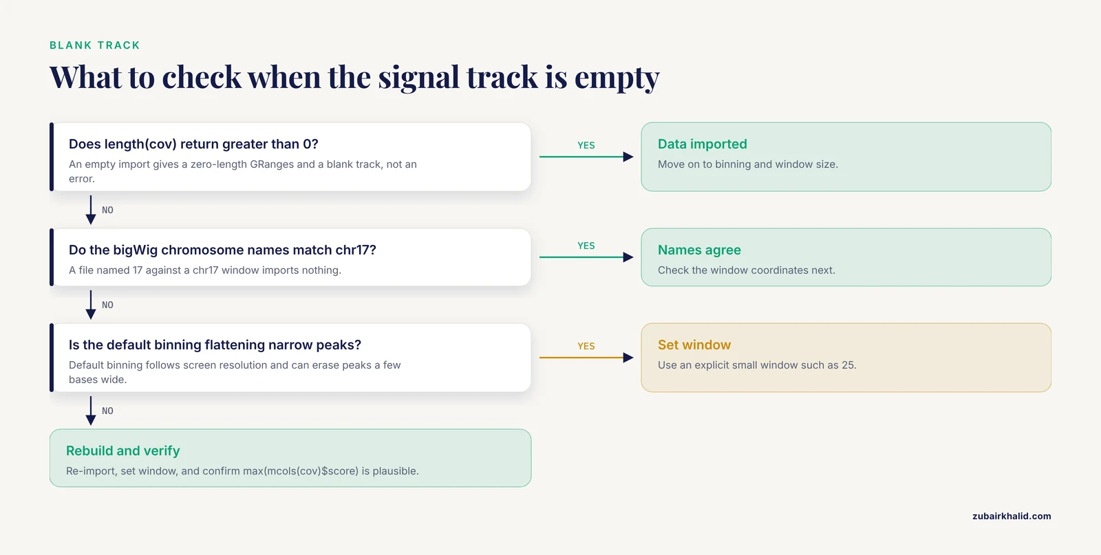
Verification should be a written step in the script, not a visual impression. Four checks cover nearly every silent failure.

First, confirm the coordinates and identifiers agree everywhere:

unique(as.character(seqnames(vr_window)))   # should print "chr17"
unique(genome(vr_window))                    # should print "hg38"
width(range(region))                         # the plotted span in bases

Second, confirm the quantitative track actually imported data rather than an empty range:

length(cov)                 # greater than 0
max(mcols(cov)$score)       # a plausible maximum, not NA

An empty import from a bigWig whose chromosomes are named 1 while your window says chr17 produces a zero-length GRanges, which then produces a blank track rather than a loud error. This is the classic quiet failure.

Third, sanity-check the gene model. Pick one transcript ID from the figure, print it with head(transcripts(edb, filter = ...)) or from your GTF, and compare its exon boundaries to what you see. A wrong annotation release is invisible in the figure but fatal in the caption.

Fourth, record the session. Write sessionInfo() output to a text file alongside the figure so any collaborator can reproduce the exact package environment. This mirrors the notebook-based verification workflow that published R tutorials across domains recommend, where each analytical step is followed by an explicit check of its output [5].

From static figures to interactive and reusable tools

Once the plotting code works, two extensions are worth the effort.

The first is an interactive wrapper. Gviz draws through the grid graphics system, so a plotTracks() call runs unchanged inside a Shiny renderPlot():

library(shiny)

ui <- fluidPage(plotOutput("locus"))

server <- function(input, output) {
  output$locus <- renderPlot({
    plotTracks(list(atr, gtrack, dtrack),
               from = 7670000, to = 7687500, chromosome = "chr17")
  })
}

shinyApp(ui, server)

This is exactly the pattern behind the yEvo Mutation Browser, which uses R Shiny to serve an interactive chromosome map, mutation categorization graphs, and a gene viewer over whole-genome sequencing results, giving users the zoom-and-ask-questions experience that static figures cannot [1]. Wrapping a Gviz pipeline in Shiny costs little because the rendering code is already written.

The second extension is packaging. Move your track construction and plotting functions, your color palettes, and any small test data into an R package with documentation and unit tests. The same argument made for packaging health economic models in R applies to visualization pipelines: structured collections of functions, data, and tests improve transparency, reduce human error, and make the work easy for collaborators to install and review [3].

Frequently Asked Questions

Can Gviz fetch data directly from UCSC or Ensembl?

Yes. UcscTrack() pulls annotation from UCSC table browsers and BiomartGeneRegionTrack() pulls gene models from Ensembl Biomart at plot time. Both require network access, and both work better for one-off exploration than for reproducible pipelines, where a cached EnsDb or a local GTF is the more stable choice.

How do I fix chromosome naming mismatches between Ensembl and UCSC data?

Convert one side with seqlevelsStyle(gr) <- "UCSC" or seqlevelsStyle(gr) <- "Ensembl" from GenomeInfoDb before building tracks. Apply the conversion to every GRanges that enters the figure, including variant ranges and imported file data.

Why is my DataTrack blank or missing peaks?

Usually the import returned no overlapping rows because of a chromosome naming mismatch, or the default binning aggregated fine structure away. Check length() on the imported GRanges first, then set an explicit small window value and confirm your window coordinates.

Can Gviz produce publication-quality figures?

Yes. Render to PDF for vector output or to PNG at 300 dots per inch, set fonts and colors through displayPars, and allocate panel space with sizes. All appearance is parameter-driven, so a style guide applied once applies to every figure in a paper.

How do I plot the same tracks across many loci?

Store your windows in a GRangesList or data frame, loop over them, subset every input to each window, and write each plotTracks() call to a separate PDF page. Keep window fixed across loci so signal aggregation is comparable.

Does Gviz work with bigWig and BAM files?

Yes, through rtracklayer. Import bigWig signal with import(bw, which = region) and pass the result to DataTrack. For BAM, import(bamFile, which = region, format = "bam") returns alignments that you can reduce into coverage with coverage() before building a DataTrack.

How is Gviz different from IGV or an R Shiny browser?

Gviz produces static, scripted, reproducible figures; IGV is an interactive desktop viewer; a Shiny application wraps scripted rendering in an interactive interface. The yEvo Mutation Browser illustrates the Shiny route, combining a chromosome map, mutation graphs, and a gene viewer for interactive exploration of sequencing results [1]. Use Gviz when the deliverable is a figure.

What annotation sources can I use for gene models?

EnsDb objects from AnnotationHub, TxDb objects from Bioconductor, or a local GTF or GFF3 imported with rtracklayer and mapped to the transcript, exon, gene, and symbol columns that GeneRegionTrack() expects. Cached EnsDb objects are the most convenient option when the workflow must run offline.

Sources

1. The yEvo Mutation Browser: Enhancing student understanding of experimental evolution and genomics through interactive data visualization.
2. How to perform a meta-analysis with R: a practical tutorial
3. Packaging cost-effectiveness models in R: A tutorial.
4. Evaluation of randomized controlled trials: a primer and tutorial for mental health researchers
5. Tutorial: guidelines for annotating single-cell transcriptomic maps using automated and manual methods