How to Fix 'No Gene Set Enriched' Errors in GSEA
By Dr. Zubair Khalid, DVM, MS, PhD ·

Gene Set Enrichment Analysis (GSEA) scores a ranked list of genes, usually ranked by a statistic such as the shrunken log2 fold change from a differential expression analysis, against curated gene sets such as the MSigDB Hallmark collections. When a run finishes and the result table comes back empty, the software is telling you one specific thing: after it intersected your ranked list with each gene set, no set passed the internal filters and produced a test statistic that survived your significance threshold. That failure almost always has a mechanical cause you can find in minutes.
The single most common cause of a "no gene set enriched" error or an empty result table is a gene identifier mismatch. Your expression matrix uses one identifier system, your gene set database uses another, and the intersection between them collapses to nearly nothing. Before you touch any statistics, run this check:
length(intersect(names(ranked_vector), unique(unlist(pathways))))If that number is small relative to your gene set universe, for example a few hundred genes out of more than ten thousand, stop. You have an identifier problem, and every downstream result is meaningless until it is fixed. This article walks through the causes of the "no gene set enriched" error from the most common to the rarest, explains the mechanism behind each failure, and gives you the commands and decisions that fix it.
Run This Diagnostic Sequence First
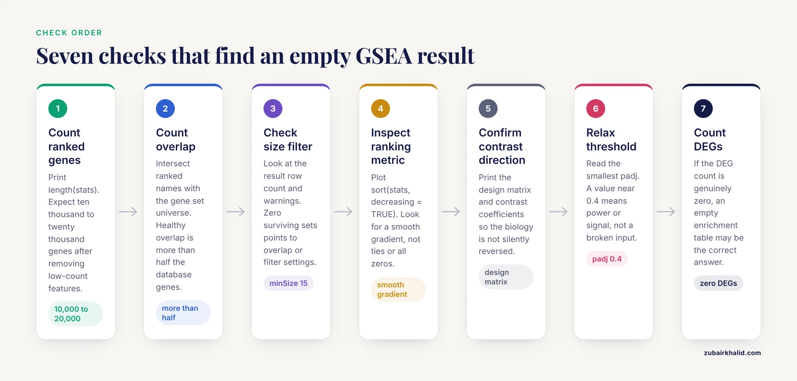
Work through these checks in order. Most empty GSEA results are resolved by step 3.
- Count the genes in your ranked list. Print
length(stats). For a typical bulk RNA-seq experiment with human or mouse annotations, this should be in the range of ten thousand to twenty thousand genes after removing low-count features. If it is in the hundreds, your input was filtered or parsed incorrectly. - Count the overlap with your gene set universe. Use the
intersectcommand shown above. A healthy overlap is typically more than half of the genes present in the gene set database for your organism. - Check how many gene sets survive the size filter. In
fgsea, look at the row count of the result object and any warnings. If zero sets survivedminSizeandmaxSize, your overlap or your filter settings are the problem. - Inspect the ranking metric. Plot
sort(stats, decreasing = TRUE). You should see a smooth gradient from strongly positive to strongly negative values. A wall of identical values, a metric that is all zeros, or a bimodal distribution with thousands of exact ties all indicate a broken input. - Confirm the direction of your contrast. Print the design matrix and the contrast coefficients from your differential expression model. A reversed contrast does not cause an empty result by itself, but it silently reverses the biology of every result you do get.
- Relax the significance threshold temporarily. Look at the unadjusted
pvalcolumn and the smallestpadjvalues. If the smallest adjusted p-value is 0.4 rather than 1.0, you have a power or signal problem rather than an input problem. - Verify that differential expression exists at all. Count your differentially expressed genes (DEGs). If the count is genuinely zero at your thresholds, enrichment failure may be the correct answer, which is covered below.
Troubleshooting Table
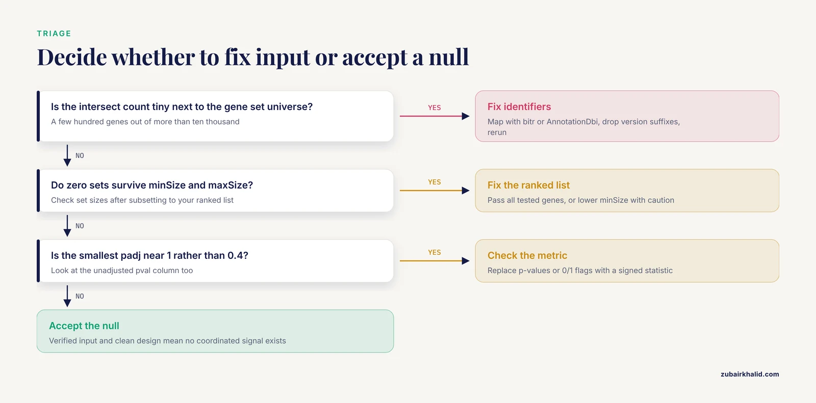
| Symptom | Likely cause | How to confirm | Fix |
|---|---|---|---|
| Zero rows in the result table | Identifier mismatch between ranked list and gene sets | intersect count is tiny compared to the gene set universe | Map identifiers with bitr, AnnotationDbi, or an official crosswalk file, then rerun |
| Zero rows, overlap looks fine | All gene sets fall outside minSize/maxSize | Print the size of each set after subsetting to your ranked list | Adjust minSize/maxSize, typically 15 and 500, and check organism |
fgsea warns about ties in preranked stats | Ranking metric has many identical values | sum(duplicated(stats)) returns a large number | Use signed, continuous statistics such as the shrunken Wald statistic rather than binarized values or raw p-values |
Result table exists but padj is 1 everywhere | No real signal, or the ranking metric is uninformative | Top of the ranked list contains housekeeping and ribosomal genes rather than biology | Recheck the differential expression model, sample groups, and contrast |
| Results appear only before FDR correction | Multiple-testing burden with a large gene set collection | Smallest raw p-values are small but padj values are not | Increase sample size, reduce the number of gene sets tested, or report suggestive results with explicit caveats |
| Enrichment is significant in the wrong direction | Reversed contrast or swapped group labels | Check the design matrix and the sign of the log2 fold change for known marker genes | Correct the contrast definition and rerun |
| Results change when genes are added or removed | Pre-filtering or ranking ties, not real biology | Compare ranked list construction across runs | Rank all tested genes with a continuous statistic, avoid hard fold-change cutoffs before ranking |
| Results fail to replicate across related datasets | Fragile, low-power finding | Compare leading-edge genes and enrichment direction across cohorts | Look for convergent pathway-level signals rather than identical set lists |
| Everything enriches, including ribosomal sets | Latent batch effect or composition artifact | Plot relative log expression per sample, check ribosomal gene behavior | Regress or remove the covariate, then rerun |
| Run errors out before producing a table | Malformed input, duplicated gene names, non-numeric statistics | str() on the ranked vector, check for factors or characters | Coerce to named numeric vector, collapse duplicates, remove missing values |
Cause 1: Gene Identifier Mismatch
This is the error to check first because it is the most common and the cheapest to fix. GSEA needs every gene in your ranked list to be comparable against the genes listed in each gene set. The comparison is a strict string match on whatever identifier system you supply. If your counts matrix carries Ensembl gene IDs with version suffixes such as ENSMUSG00000012345.12 and your gene sets carry plain Entrez gene IDs, the intersection is empty and every set is discarded.
The mismatch takes several common forms:
- Different identifier systems. Ensembl IDs, Entrez gene IDs, HGNC symbols, UniProt accessions, and probe identifiers are all different namespaces. Gene set databases are most commonly distributed with Entrez IDs or official symbols.
- Version suffixes. Ensembl IDs from recent GTF releases carry a
.Nsuffix that breaks matching against versionless gene sets. - Capitalization. Human symbols are uppercase, mouse symbols are capitalized first letters only. Matching
TnfagainstTNFfails. - Protein and metabolite identifiers. If you are running enrichment on proteomics or metabolomics data, the identifier problem is worse because gene set databases are annotated at the transcript level and require cross-omics mapping [1].
The fix is to map everything into one namespace before ranking. In R, the clusterProfiler function bitr or an org.Xx.eg.db annotation package does this for standard model organisms:
library(clusterProfiler)
library(org.Hs.eg.db)

mapped <- bitr(geneID = rownames(counts_df),
               fromType = "ENSEMBL",
               toType = "ENTREZID",
               OrgDb = org.Hs.eg.db)
Drop Ensembl version suffixes with a regular expression such as sub("\\..*$", "", ids) before mapping. After mapping, collapse duplicate rows by taking the feature with the largest mean expression or the smallest p-value, because one gene symbol can map from several Ensembl IDs. Then rebuild the ranked vector and verify the overlap count again.
For multi-omics projects where you want transcript, protein, and metabolite layers analyzed together, purpose-built packages handle the identifier mapping as part of the workflow. The multiGSEA package, for example, queries eight pathway databases, supports eleven organisms, and includes comprehensive mapping of transcript, protein, and metabolite identifiers so that each omics layer can be projected onto a common gene set space [1].
Cause 2: Gene Set Size Filtering Removes Everything
GSEA filters gene sets by size twice. The database itself sets minimum and maximum set sizes, and then the software intersects each set with the genes present in your ranked list and applies the filter again. If the intersection shrinks a set below the minimum, the set is silently dropped.
The standard defaults are a minimum of 15 and a maximum of 500 genes per set. These defaults exist for statistical reasons. Sets smaller than about 15 genes produce unstable enrichment scores and worthless permutation p-values. Sets larger than 500 genes are so broad that an enrichment result is hard to interpret and the running-sum statistic behaves poorly.
The failure mode looks like this: your ranked list contains only, say, 2,000 genes because you pre-filtered aggressively, most Hallmark sets intersect down to fewer than 15 genes, and the run returns nothing. Confirm it directly:
set_sizes <- sapply(pathways, function(p) sum(p %in% names(ranks)))
summary(set_sizes[set_sizes > 0])
table(set_sizes >= 15 & set_sizes <= 500)
Two fixes apply, in order of preference. First, fix the ranked list so it contains all tested genes, which is what GSEA expects (see Cause 4). Second, if your experiment genuinely limits you to a short gene list, lower minSize with the understanding that small sets give fragile results, or switch to an over-representation analysis (ORA), which is designed for a list of significant genes rather than a full ranked list.
Also confirm that the gene set database matches your organism. Loading human MSigDB sets against a mouse, rat, or chick ranked list guarantees that every set fails the size filter. Tools differ in whether they expect Entrez IDs or symbols per organism, so check the documentation of the specific database source you are using.
Cause 3: The Ranking Metric Is Broken
GSEA ranks every gene by a single signed, continuous statistic and computes an enrichment score (ES) from a running sum through that ranking. The normalized enrichment score (NES) is then compared against a null distribution built by permuting or resampling the labels. Everything downstream depends on the quality of that ranking metric. A broken metric produces either an empty result table or, worse, confident nonsense.
The most common broken metrics are:
- Raw p-values or adjusted p-values. These are bounded between 0 and 1 and carry no direction. Every gene appears to be "up". GSEA needs signed values.
- Binarized or thresholded values. If you passed a 0/1 DEG indicator as the statistic, the running sum degenerates. Report the number of ties: ``
r sum(duplicated(stats))`` - Unshrunken fold changes from low-count genes. Genes with tiny counts produce extreme, noise-driven fold changes that dominate both ends of the ranking. Use moderated or shrunken statistics such as those from
limmaorDESeq2rather than raw log2 fold changes alone. - A metric that is effectively zero everywhere. If your two groups are biologically identical or your contrast is wrong, the ranked gradient is flat, permutation nulls match the observed data, and nothing is enriched. This is the honest failure: the analysis is telling you the data contain no coordinated signal.
The fgsea package explicitly warns "There are ties in the preranked stats" when duplicate values exist in the statistic. Treat that warning as an instruction to fix the input, not as noise to ignore. Ties break the ordering of the running sum and degrade the permutation null.
The correct input for a standard RNA-seq GSEA is the signed Wald statistic or shrunken log2 fold change for every gene that passed your expression filter, named by Entrez ID or symbol:
res <- results(dds, contrast = c("condition", "treated", "control"))
stats <- res$stat
names(stats) <- mapIds(org.Mm.eg.db,
                       keys = rownames(res),
                       keytype = "ENSEMBL",
                       column = "ENTREZID")
stats <- stats[!is.na(names(stats))]
stats <- sort(stats, decreasing = TRUE)
Cause 4: Overly Aggressive Pre-Filtering
A frequent RNA-seq error is running GSEA on a list of significant DEGs, or on a matrix filtered down to a few thousand variable genes, and then wondering why the result looks wrong or empty. GSEA was designed to use the full ranked universe. Its strength is that it detects coordinated shifts of modest magnitude across many genes, which single-gene threshold tests miss. Comparative evaluations have shown that GSEA can detect weak deregulation signals that stricter threshold-based approaches miss, and that Fisher's exact test on a DEG list performs markedly worse in simulation studies [2].
When you pre-filter to DEGs, two things go wrong. The ranked gradient collapses because every gene above your cutoff has essentially the same effective rank position. And the size filter from Cause 2 kicks in, because the intersection of gene sets with a short list falls below the minimum set size.
The practical rule: pass GSEA all genes that survived basic expression filtering, such as genes with at least a small count threshold across samples, ranked by a continuous signed statistic. Save the DEG list for over-representation analysis, which is the method designed for it. Running both on the same dataset is standard practice because they answer related but different questions.
The same principle extends beyond RNA-seq. In a label-free proteomics study of retinal responses to induced refractive error, researchers identified differentially abundant proteins with moderated t-tests at a fold change of 1.5 or greater and adjusted p below 0.05, then ran GSEA on the protein-level measurements to examine pathway-level expression [3]. The point is not the specific cutoffs, which belong to that study, but that the enrichment input was built from the quantitative analysis output at the correct feature level, with identifiers mapped appropriately, rather than from a short filtered list.
Cause 5: Weak or Absent Biological Signal
Sometimes the pipeline is correct and the answer is that the data contain no enrichment. Two distinct situations hide here, and they require different responses.
The first situation is a genuinely null result. If your perturbation has no transcriptional effect, your sample size is too small, or your comparison is between groups that differ only in ways the transcriptome does not reflect, an empty enrichment table is the correct output. Do not keep tuning parameters until something turns significant. That path leads to the false-positive problem described later in this article.
The second situation is real but diffuse signal. GSEA exists precisely for cases where no individual gene crosses the significance threshold but a set of genes shifts coordinately. In a study of fatigue in primary Sjögren's syndrome, no genes were individually associated with fatigue, yet GSEA identified 19 enriched metabolic pathways in the high-fatigue group, driven by a subset of 55 genes, and that gene subset improved classifier performance [4]. Conversely, in a cross-disease comparison of Gaucher disease and common variable immunodeficiency, only 2 genes were differentially expressed between inflammatory and non-inflammatory CVID at an adjusted p below 0.05, while 143 Reactome pathways remained robust to demographic adjustment [5]. Both results illustrate the same principle: a near-empty DEG table does not imply an empty enrichment table, and a rich enrichment table does not imply many DEGs.
How do you tell these situations apart? Look at the observed enrichment score (ES) and the NES before looking at p-values. If NES values hover near 1.0 with p-values near 0.5 across the whole collection, the ranked list carries no set-level structure. If NES values are moderately large but FDR fails, you have a power problem, which points to sample size, permutation number, or the number of gene sets tested rather than the input data.
Cause 6: Statistical Thresholds, Permutations, and Power
Multiple-testing correction over a large gene set collection is unforgiving. Testing thousands of sets means the FDR (false discovery rate) adjustment inflates the required evidence for each individual set. In a pathway-based genome-wide association study of plasma adiponectin levels, the Rac1 pathway was associated with the trait at a raw empirical p below 0.001 with FDR 0.008, while a quantitative version of the same pathway analysis produced a raw empirical p of 0.001 but failed multiple-testing correction at FDR 0.11 [6]. The signal was real in both analyses. The threshold alone decided whether it was reported.
When your result table has rows but nothing survives FDR:
- Increase permutations. The classical GSEA default uses 1,000 permutations. With very small raw p-values, the resolution of the null distribution limits what FDR correction can detect. More permutations give finer nulls. Modern implementations such as
fgseause a multilevel approach that avoids this resolution ceiling for small p-values, which is one reason results can differ between tools. - Reduce the number of sets tested. Testing a focused collection, such as Hallmark sets or sets relevant to your tissue, reduces the correction burden compared to testing every set in a comprehensive database.
- Increase sample size. Enrichment power tracks the quality of the underlying ranking statistic, which tracks the precision of your differential expression model. No enrichment setting compensates for a noisy ranking.
- Report the full distribution. When nothing passes FDR, report the top sets by NES with their p-values and say so explicitly, rather than reporting nothing at all. This is standard, honest practice and lets readers judge suggestive signals.
Cause 7: Design Errors, Outliers, and Hidden Covariates
An empty or nonsensical enrichment result can be the first visible symptom of a problem upstream in the statistical design. Regression diagnostics applied to gene set analysis can identify outlying or influential samples and data-entry errors, demonstrated on an acute lymphoblastic leukemia dataset where residuals aggregated by chromosomal location flagged problematic samples and revealed hyperdiploidy as a major hidden driver of expression [7]. The lesson generalizes: inspect your samples before trusting your gene sets.
Practical checks that catch the common design failures:
- Verify the design matrix. Print it. Confirm that group labels, batches, and covariates line up with the sample metadata file, and that the contrast names the groups in the order you intend.
- Look for outliers. Principal component plots and per-sample relative log expression reveal swapped samples and failed libraries. Remove or investigate outliers with a stated, pre-specified rule rather than by outcome.
- Check for hidden structure. Supposedly identical model organisms and cell lines carry real sequence and environmental variation that can confound an analysis, a phenomenon documented even in nominally isogenic C. elegans strains where unanticipated mutations and strain differences complicated the interpretation of pathway defects [8]. If your groups differ in batch, sex, passage number, or sequencing lane, include those terms in the model or the ranking statistic will reflect them instead of your treatment.
- Watch for composition artifacts. If one condition contains more of a particular cell type, whole-organism or bulk tissue data will show enrichment of that cell type's signature genes. Ribosomal and mitochondrial sets enriching prominently, a pattern that appears repeatedly in problematic GSEA runs [9], is a classic flag for a composition or quality artifact rather than a treatment effect.
Cause 8: Platform and Data-Type Mismatch
GSEA was built for gene expression ranked lists. Applying it unchanged to other data types introduces failure modes that produce empty results or biased ones.
In DNA methylation analysis, standard GSEA methods struggle with probe dependency, probe number bias, and the complexity of gene-probe mapping, because CpG probes differ in number per gene and correlate with each other, which biases enrichment results and reduces power [10]. The remedy is a method built for the platform that aggregates probe-level signals to the gene level while correcting for these dependencies, rather than feeding raw probe statistics into a gene-oriented tool. The same logic applies to proteomics, where protein identifiers and abundance distributions differ from transcripts, and to single-cell data, where pseudobulk aggregation is usually the appropriate input.
Data type matters for method choice as well. In genetic association data, comparisons on SNP data showed that GSEA and Fisher's exact test lack power and robustness relative to a set-based sum statistic, which found more significant gene sets with better type I error control [11]. If your data are SNP-level summary statistics rather than expression values, use a method designed for that input.
Finally, if your question spans multiple omics layers, a single-layer GSEA that comes back empty may simply reflect that the signal lives in another layer. Multi-omics enrichment frameworks combine per-layer enrichment scores into a composite measure precisely because individual layers can be too noisy or too sparse to yield significant sets alone [1].
Choosing an Alternative or Complementary Method
When GSEA returns nothing, run a second method before concluding that no biology exists. Different methods answer different questions and have different power profiles.
- Over-representation analysis (ORA). Use a list of significant genes and test whether any gene set is overrepresented among them, typically with a hypergeometric or Fisher's exact test. This is the correct method when you have a short DEG list, and it frequently produces results when a misconfigured GSEA does not. Comparative simulations found Fisher's exact test markedly worse than GSEA and random-sets approaches for detecting set-level deregulation, so treat ORA as a complement rather than a replacement [2].
- GSVA. Gene Set Variation Analysis computes a pathway activity score per sample rather than per contrast, which supports pathway-level modeling across continuous phenotypes and sample-level clustering. Radiogenomic studies commonly run GSEA and GSVA side by side on the same cohorts to capture both contrast-level and sample-level pathway activity [12].
- CERNO and other fast alternatives. If you are using
fgseaand suspect algorithm-specific behavior, a different algorithm on the same ranked list is an inexpensive robustness check. In evaluations of GSEA false positives, CERNO was used as an alternative implementation to compare against [9]. - Correlation-aware gene set tests. Most gene set methods, GSEA included, treat genes in a set as independent, which they are not. Variance component approaches such as TEGS model the correlation among genes within a set explicitly and can improve power while protecting the type I error rate [13].
- Multi-omics enrichment. When transcriptomics alone is unrevealing, combining layers can recover pathway signals that no single layer shows [1].
A reasonable routine for a troubled RNA-seq dataset is ORA on the DEG list, GSEA on the full ranked list, and GSVA for sample-level scores. Agreement across methods, especially agreement on enrichment direction, is strong evidence that a finding is real.
Guarding Against the Opposite Problem
Once your pipeline produces results, remember that "no gene set enriched" and "many gene sets enriched" can both be artifacts. A controlled study using zebrafish embryo expression data, where vehicle-treated groups should show no true treatment differences, quantified false-positive enrichment directly. False positives from the fgsea algorithm increased with pool and sample size and were most frequent in simulations that generated zero DEGs, with ribosomal gene sets enriched with the highest frequency. The authors described two distinct mechanisms, both most likely to produce significant sets when expression differences are particularly low [9].
The operational takeaways for your own runs: treat a large harvest of significant sets from a dataset with few or no DEGs as suspect. Suspect ribosomal, mitochondrial, and spliceosomal sets that top every comparison regardless of biology. And validate: pathway-level findings should replicate in direction across independent datasets or related experimental conditions, as demonstrated in a Gaucher disease framework where enriched Reactome pathways were carried through leave-one-patient-out testing, expression-scale sensitivity analysis, and external validation before being called robust [5]. A finding that survives that gauntlet is worth reporting. One that appears only in a single configuration of a single tool is not.
Common Mistakes and Limitations
- Running GSEA on a DEG list. This converts GSEA into a degenerate version of itself, destroys the ranked gradient, and usually triggers the size filter. GSEA takes all genes, ranked. ORA takes the DEG list. Do not cross them.
- Interpreting a reversed NES. Sign follows your contrast definition. A negative NES for "treated versus control" means the set is enriched toward control. Always state the contrast in your figure legends.
- Chasing significance by adjusting thresholds. Lowering
minSize, raisingmaxSize, or loosening FDR until something appears is not a fix. It converts a null result into a likely false positive, which is precisely the regime where GSEA false positives cluster [9]. - Ignoring the tie warning. Duplicate values in the ranking statistic degrade both the enrichment score and the null. Fix the metric instead of suppressing the warning.
- Trusting a single tool's output. Permutation schemes, tie handling, and p-value estimation differ between the GSEA desktop application,
fgsea, andclusterProfiler. Different results are expected for borderline sets. Concern yourself with sets that are strongly enriched and consistent across tools. - Forgetting that GSEA assumes gene-level independence within sets. Genes in pathways are correlated, and methods that model that correlation explicitly can behave differently from GSEA on the same data [13]. Differences between methods are information, not noise.
- Overreading pathway names. Enrichment of "MYC targets" tells you a coordinated expression program is present, not that MYC itself is activated. Follow up with leading-edge gene inspection.
- Expecting replication of exact set lists. Independent cohorts routinely show convergent pathway-level signals with only partial overlap in the specific sets called significant, and context-dependent replication is the norm even in well-powered studies [5]. Look for direction and mechanism, not identical output.
One limitation applies to any computational workflow. Pipeline fixes establish that an analysis was performed correctly. Whether an enrichment finding reflects real biology in your specific system requires domain judgment, and individual datasets deserve expert review before conclusions are drawn from them.
Prevention Practices
Adopt these habits and the "no gene set enriched" error becomes a rare, quickly diagnosed event rather than a day-long crisis.
- Standardize identifiers at the start of every project. Convert all feature identifiers to one namespace, ideally Entrez IDs or official symbols, in a single documented script that runs before any analysis.
- Build one reusable GSEA input function. A function that takes a differential expression result object and returns a sorted, named, deduplicated numeric vector eliminates most input errors permanently.
- Assert before you analyze. Add checks to your script: ranked list length, overlap fraction with the gene set universe, number of surviving sets, and tie count. Fail loudly with informative messages.
- Record the configuration. Save the gene set version, organism,
minSize,maxSize, permutation settings, and the exact contrast definition alongside the results. Unreproducible enrichment analyses waste more time than broken ones. - Run two methods by default. GSEA on the ranked list plus ORA on the DEG list covers the complementary failure modes of each. Agreement strengthens conclusions, disagreement directs debugging.
- Validate enrichment direction with marker genes. Before publishing or interpreting a result, confirm that known positive-control sets enrich in the expected direction. If glycolysis genes go down in a hypoxia experiment, your contrast is reversed.
- Pre-specify your thresholds. Decide on FDR and set size limits before looking at results, and report all configurations you tried. This protects you from your own enthusiasm and from reviewers who will ask.
- Keep the DEG count in the report. Report the number of DEGs and the number of enriched sets together, because the relationship between them is diagnostic. Many DEGs with no enrichment suggests a configuration problem. Few DEGs with strong enrichment is the classic GSEA use case [4].
Frequently Asked Questions
Why does GSEA return no gene sets even though I have hundreds of DEGs?
You almost certainly ran GSEA on the DEG list instead of the full ranked gene universe. GSEA requires all tested genes ranked by a continuous signed statistic. Feed it the complete filtered matrix ranked by the Wald statistic or shrunken fold change, and use the DEG list for over-representation analysis instead.
What does the "ties in the preranked stats" warning mean?
Your ranking statistic contains duplicate values, usually from p-values, binarized indicators, or heavily filtered input. Ties break the ordering that the running-sum statistic depends on. Replace the metric with a signed, continuous value such as the Wald statistic for every gene.
What minSize and maxSize values should I use for GSEA?
The standard defaults are 15 and 500 genes per set after intersection with your ranked list. Sets below 15 genes give unstable statistics and sets above 500 genes are too broad to interpret. Change these only when your data genuinely require it, and report what you used.
Can GSEA find real pathways when no individual genes are significant?
Yes. GSEA was designed for coordinated, modest shifts across many genes that no single-gene test detects. Studies have documented strong pathway-level enrichment alongside near-empty DEG lists, which is exactly the situation GSEA handles better than threshold-based methods.
Why do clusterProfiler, fgsea, and the GSEA desktop app give different results?
They use different permutation schemes, tie handling, and p-value estimation methods, so borderline sets will differ. Strongly enriched sets with large NES values should agree. Check that all three received the same identifiers, the same ranked metric, and the same size filters before comparing.
Is "no gene set enriched" ever the correct answer?
Yes. If the input is verified correct, the ranking metric is sound, and the design is clean, an empty result means the data contain no detectable coordinated pathway signal. Do not keep adjusting parameters until something crosses the threshold, because that manufactures false positives.
Should I use pval or padj when reporting GSEA results?
Report padj, the FDR-adjusted value, as the primary criterion for calling a set significant, and include the raw p-value and NES for context. Multiple-testing correction across thousands of sets is mandatory, and raw p-values alone will fill your table with expected false positives.
My GSEA results do not replicate in a second dataset. Is the finding wrong?
Not necessarily wrong, but unconfirmed. Independent cohorts frequently show convergent enrichment direction and overlapping leading-edge genes without identical significant set lists. If the direction, the leading-edge genes, and the biological theme agree across datasets, the finding is credible. If nothing aligns, treat the original result as fragile.
Sources
- multiGSEA: a GSEA-based pathway enrichment analysis for multi-omics data.
- Comparative study of gene set enrichment methods.
- Short term optical defocus perturbs normal developmental shifts in retina/RPE protein abundance.
- A Transcriptional Signature of Fatigue Derived from Patients with Primary Sjögren's Syndrome.
- Pathway-level transcriptional convergence between Gaucher disease and Common variable immunodeficiency reveals concordant interferon and antigen-processing signatures.
- Pathway-Based Genome-wide Association Studies Reveal That the Rac1 Pathway Is Associated with Plasma Adiponectin Levels.
- Gene set enrichment analysis using linear models and diagnostics.
- Natural and unanticipated modifiers of RNAi activity in Caenorhabditis elegans.
- Gene Set Enrichment Analysis in Zebrafish Embryos Is Susceptible to False-Positive Results in the Absence of Differentially Expressed Genes.
- Efficient gene set analysis for DNA methylation addressing probe dependency and bias.
- Comparing gene set analysis methods on single-nucleotide polymorphism data from Genetic Analysis Workshop 16.
- Identifying Associations between DCE-MRI Radiomic Features and Expression Heterogeneity of Hallmark Pathways in Breast Cancer: A Multi-Center Radiogenomic Study.
- Gene set analysis using variance component tests.