GSEA in R with clusterProfiler: Step-by-Step Tutorial
By Dr. Zubair Khalid, DVM, MS, PhD ·

By the end of this GSEA in R with clusterProfiler tutorial you will be able to take a differential expression table, build a ranked gene list, run gene set enrichment analysis (GSEA) against Gene Ontology (GO), KEGG, and MSigDB gene sets, interpret normalized enrichment scores and leading edge genes, and produce the standard figures for a report or paper. Everything runs locally in R on a laptop in minutes.
You need three things on hand:
- R 4.3 or newer, with an internet connection for package installation and KEGG downloads
- A gene count matrix with samples in two conditions, plus a sample sheet
- Roughly 30 minutes for the first full run
clusterProfiler is the standard R package for this work. It provides over-representation analysis (ORA) and GSEA behind consistent interfaces, along with a large set of visualizations that ranges from bar plots and dot plots to enrichment maps [1]. Protocol material written for bench scientists describes the same two method families, ORA and functional class scoring (FCS), run against the GO, KEGG, and Reactome knowledge bases in R [2]. This tutorial covers the FCS side, GSEA, and every decision that changes your results.
What GSEA Does and When to Use It
ORA versus functional class scoring
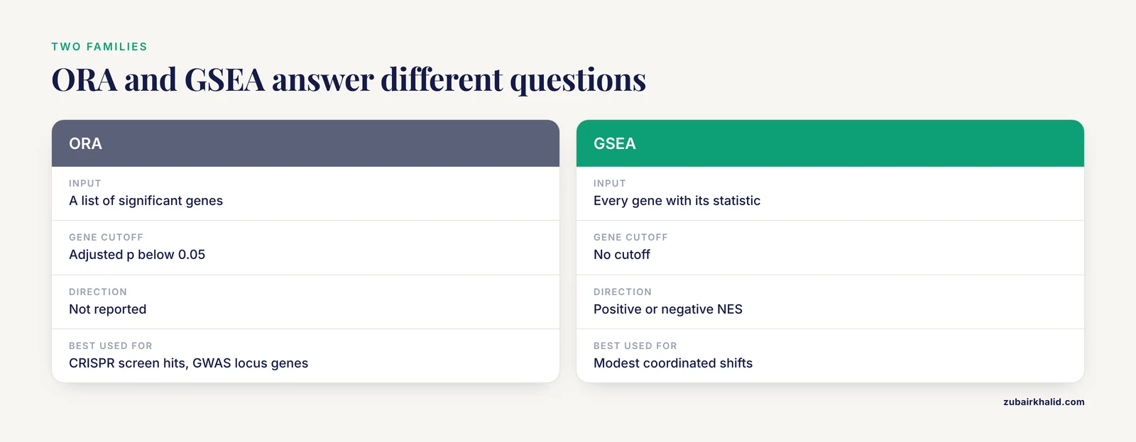
Functional enrichment analysis comes in two families. ORA takes a list of genes you already called significant, for example adjusted p below 0.05, and asks whether known gene sets appear in that list more often than chance expects. FCS keeps every gene in the experiment and uses its statistic directly, with no cutoff. Protocol literature for bench scientists covers both families and their R implementations in detail [2].
GSEA is the most widely used FCS method. The algorithm has four moves. First, rank all genes from most positive to most negative by a metric such as the DESeq2 Wald statistic. Second, walk down the list and compute a running sum that increases when you meet a gene from the set and decreases when you do not, weighted by the magnitude of the metric. The maximum deviation from zero is the enrichment score (ES). Third, estimate a p-value by permutation and normalize the ES against the permutation distribution to get the normalized enrichment score (NES), which is comparable across gene sets. Fourth, adjust p-values across all tested sets, almost always with Benjamini-Hochberg false discovery rate (FDR) control. The genes at or before the point of maximum deviation form the leading edge, the subset that actually drives the signal.
When GSEA is the better choice
Choose GSEA when shifts are modest and coordinated, when no principled cutoff exists, or when direction matters, because a positive NES places a set at the top of the list and a negative NES places it at the bottom. ORA remains the right tool when your input is a list from somewhere else, such as CRISPR screen hits or GWAS locus genes. Published pipelines use both. Quantitative proteomics protocols run ORA and GSEA side by side on ranked protein statistics [3], and enrichment analysis in general is described as a cornerstone for putting transcriptomics and proteomics data into biological context [1].
Install R, Bioconductor, and the clusterProfiler Stack
R for bioinformatics means R plus Bioconductor, the open software project that hosts clusterProfiler, DESeq2, and the annotation databases used here. Every Bioconductor tutorial starts the same way, with BiocManager. Bioconductor issues a stable release every six months, so record your versions as you go.
install.packages("BiocManager")
BiocManager::install(c(
  "clusterProfiler",   # GSEA engine and ORA
  "enrichplot",        # visualization
  "fgsea",             # fast GSEA implementation used under the hood
  "DESeq2",            # differential expression
  "org.Hs.eg.db",      # human gene annotation
  "msigdbr",           # MSigDB gene sets as data frames
  "ggplot2"
))
Load the packages and print the session record you will paste into your methods section:
library(clusterProfiler)
library(enrichplot)
library(DESeq2)
library(fgsea)
library(msigdbr)
library(org.Hs.eg.db)

sessionInfo()
Two version notes before you start. clusterProfiler 4.x computes GSEA through fgsea's adaptive multilevel permutation algorithm, controlled by the eps argument, while older 3.x versions used a fixed permutation count set by nPerm. The msigdbr package renamed its category argument to collection in version 10. The code below shows the current forms and flags the older ones where it matters.
Step 1: Build a Ranked Gene List From Differential Expression
Run differential expression
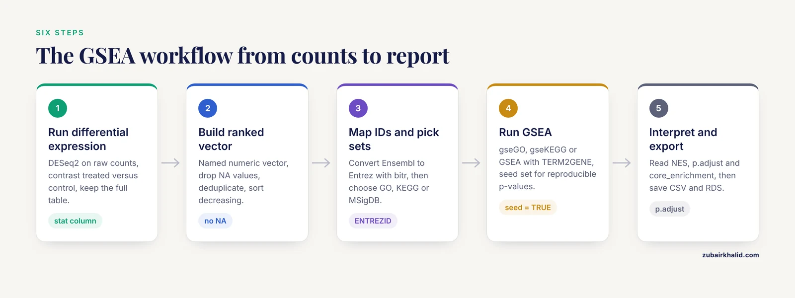
GSEA consumes the complete ranked list, so start from the full differential expression table, not a filtered one. This example uses raw counts with samples in two conditions, control and treated.
counts  <- read.csv("counts.csv", row.names = 1)
coldata <- read.csv("coldata.csv", row.names = 1)
# counts.csv: genes as rows, samples as columns, raw integer counts
# coldata.csv: one row per sample, a condition column with control and treated

dds <- DESeqDataSetFromMatrix(
  countData = round(counts),
  colData   = coldata,
  design    = ~ condition
)
dds <- DESeq(dds)
res <- results(dds, contrast = c("condition", "treated", "control"))
The contrast order matters. With treated listed first, positive values mean up in treated. Reverse the order and every downstream NES flips sign.
Turn results into a sorted, named vector
The stat column of the DESeq2 results holds the Wald statistic, the log2 fold change divided by its standard error. It is the usual ranking metric because it combines effect size with measurement confidence and produces few ties. Ranking by p-value is a mistake, p-values saturate near zero, carry no direction, and tie thousands of genes together. Ranking by raw log2 fold change is acceptable but noisy for low-count genes, and if you prefer it, shrink the estimates first with lfcShrink.
ranked <- res$stat
names(ranked) <- rownames(res)
ranked <- ranked[!is.na(ranked)]              # drop genes without a statistic
ranked <- ranked[!duplicated(names(ranked))]  # one entry per gene
ranked <- sort(ranked, decreasing = TRUE)     # most positive on top
head(ranked)
Expected output, with your own identifiers and values:
ENSG00000141510 ENSG00000121879 ENSG00000179094 ENSG00000108654 ENSG00000110958 ENSG00000076984
          9.412           8.873           8.415           7.996           7.742           7.501
A valid input has three properties, every gene carries a name, the vector is numeric with no NA values, and it is sorted decreasingly. Keep the full list. Tens of thousands of genes is normal, and GSEA uses all of them.
Step 2: Convert Gene IDs and Prepare Gene Sets
Map everything to one identifier space
Annotation databases, KEGG, and MSigDB all work best with Entrez IDs (ENTREZID). If your counts use Ensembl gene IDs or symbols, convert once:
ids <- bitr(
  gene     = names(ranked),
  fromType = "ENSEMBL",
  toType   = "ENTREZID",
  OrgDb    = org.Hs.eg.db
)
bitr reports what it could not convert, in the package's own wording:
Warning message:
22% of input gene IDs are fail to map...
Losing some Ensembl IDs is normal, and the mapping is many-to-one in places. Rebuild the ranked vector on Entrez IDs, keeping the most extreme statistic when two inputs map to the same Entrez ID:
ranked_df <- data.frame(ENSEMBL = names(ranked), stat = as.numeric(ranked))
ranked_df <- merge(ranked_df, ids, by = "ENSEMBL")
ranked_df <- ranked_df[order(ranked_df$stat, decreasing = TRUE), ]
ranked_vec <- ranked_df$stat
names(ranked_vec) <- ranked_df$ENTREZID
ranked_vec <- ranked_vec[!duplicated(names(ranked_vec))]
Pick the gene set source
Three routes cover almost every project.
| Function | Gene sets | You supply | Best for |
|---|---|---|---|
| gseGO | GO BP, MF, CC from an OrgDb | geneList, OrgDb | Human and model organisms |
| gseKEGG | KEGG pathways, downloaded live | geneList, organism code | Pathway-level interpretation |
| GSEA() | Any term-to-gene table | geneList, TERM2GENE | MSigDB, custom sets, non-model species |
Route A, GO. The OrgDb carries the gene sets internally, so there is nothing else to prepare:
ego <- gseGO(
  geneList      = ranked_vec,
  OrgDb         = org.Hs.eg.db,
  ont           = "BP",
  keyType       = "ENTREZID",
  minGSSize     = 15,
  maxGSSize     = 500,
  pvalueCutoff  = 0.05,
  pAdjustMethod = "BH",
  seed          = TRUE,
  nproc         = 4
)
Route B, KEGG. gseKEGG downloads current KEGG data, so it needs internet. Find your organism code first:
search_kegg_organism("human")   # kegg code: hsa

kkegg <- gseKEGG(
  geneList     = ranked_vec,
  organism     = "hsa",
  minGSSize    = 15,
  maxGSSize    = 500,
  pvalueCutoff = 0.05,
  seed         = TRUE
)
The organism argument wants the three-letter KEGG code, hsa for human, mmu for mouse, dme for fly. Passing "human" fails. Setting use_internal_data = TRUE uses a bundled KEGG.db copy that is years out of date, so prefer the online download.
Route C, MSigDB or your own GMT. MSigDB ships as a data frame through msigdbr, and the Hallmark collection (H) is a good first target with roughly 50 curated, nonredundant sets:
msig_h <- msigdbr(species = "Homo sapiens", collection = "H")
# msigdbr older than version 10: msigdbr(species = "Homo sapiens", category = "H")

t2g <- unique(msig_h[, c("gs_name", "entrez_gene")])

gse_h <- GSEA(
  geneList     = ranked_vec,
  TERM2GENE    = t2g,
  minGSSize    = 15,
  maxGSSize    = 500,
  pvalueCutoff = 0.05,
  seed         = TRUE,
  nproc        = 4
)
TERM2GENE is a two-column data frame, term first, gene second. For a custom GMT file, the same two columns come from fgsea's reader:
pathways <- fgsea::gmtPathways("my_pathways.gmt")
t2g <- data.frame(
  term = rep(names(pathways), lengths(pathways)),
  gene = unlist(pathways, use.names = FALSE)
)
Non-model organisms
A missing OrgDb and KEGG code does not block you. Build a term-to-gene table from your own annotation, orthology mapping, or domain prediction, then call GSEA() with TERM2GENE. That is exactly how species-specific platforms get built. The ShEnrich resource for penaeid shrimp assembled GMT libraries for KEGG and GO across five farmed species and ran its enrichment analysis with clusterProfiler [4]. The same pattern works for any organism where you can produce a gene-to-pathway table. For human work that wants Reactome instead of KEGG, the ReactomePA package provides gseReactome with the same interface.
Step 3: Run GSEA in R with clusterProfiler
The call and what the console tells you
A healthy run prints a short sequence:
using 'fgsea' for GSEA calculation, please cite Korotkevich et al (2019).

preparing geneSet...
GSEA analysis...
leading edge analysis...
done...
The first line credits fgsea, the package doing the permutation mathematics. If the run ends immediately with
no term enriched under specific organism/datasetthen nothing passed the cutoffs, which almost always means an identifier mismatch or a cutoff problem, covered in the mistakes section.
Inspect the result table:
head(as.data.frame(gse_h))Illustrative output from a treated versus control example, your numbers will differ:
                               ID                             Description setSize enrichmentScore    NES   pvalue  p.adjust
1           HALLMARK_E2F_TARGETS                     HALLMARK_E2F_TARGETS     197           0.512  2.874  1.2e-09   4.6e-08
2         HALLMARK_G2M_CHECKPOINT                   HALLMARK_G2M_CHECKPOINT     198           0.486  2.711  4.1e-09   7.9e-08
3          HALLMARK_MYC_TARGETS_V1                  HALLMARK_MYC_TARGETS_V1     199           0.452  2.583  2.2e-08   2.8e-07
4                  HALLMARK_HYPOXIA                          HALLMARK_HYPOXIA     186          -0.401 -2.314  3.0e-06   2.9e-05
5 HALLMARK_TNFA_SIGNALING_VIA_NFKB        HALLMARK_TNFA_SIGNALING_VIA_NFKB     198           0.388  2.241  8.9e-06   6.8e-05
6   HALLMARK_INFLAMMATORY_RESPONSE          HALLMARK_INFLAMMATORY_RESPONSE     190           0.371  2.183  1.5e-05   9.6e-05
Key parameters
| Argument | What it controls | Sensible starting value |
|---|---|---|
| geneList | The named, decreasingly sorted numeric vector to test | DESeq2 stat column |
| TERM2GENE | Two-column term-to-gene map, term first | From msigdbr, a GMT, or your annotation |
| minGSSize | Sets with fewer genes are skipped | 15 |
| maxGSSize | Sets with more genes are skipped | 500 |
| pvalueCutoff | Cutoff on the adjusted p-value for returned rows | 0.05, or 1 to inspect everything |
| pAdjustMethod | Multiple testing correction across sets | "BH" |
| eps | Boundary for fgsea's adaptive permutation algorithm | Leave the default unless you need extremely small p-values |
| scoreType | Which enrichment directions are tested | Leave the default for standard two-sided GSEA |
| seed | Reproducible permutation handling | TRUE, with set.seed() before the call |
| nproc | Number of parallel workers | 4 on a typical machine |
Three parameters change results the most. minGSSize and maxGSSize bound the set sizes tested, tiny sets give unstable scores built from a handful of genes and huge sets are too diffuse to interpret, so 15 to 500 is a defensible default range. pvalueCutoff filters returned rows on the adjusted p-value. pAdjustMethod defaults to Benjamini-Hochberg, which controls the false discovery rate across the thousands of sets tested at once. The running sum itself is weighted by the metric raised to the exponent argument, which defaults to 1, the original GSEA weighting.
Practical tips
- Run one quick pass with pvalueCutoff = 1 and minGSSize = 5 to confirm identifiers are matching, then tighten for the real run.
- Call set.seed(123) before the analysis and pass seed = TRUE, permutations are random and unseeded p-values wobble in the third decimal.
- Save the result object with saveRDS, every plot in Step 5 takes it as input.
Step 4: Interpret NES, p.adjust, and the Leading Edge
Reading the columns
- enrichmentScore (ES), the signed maximum of the running sum for that set
- NES, the ES normalized against the permutation distribution, the number you compare across sets
- pvalue and p.adjust, the permutation p-value and its Benjamini-Hochberg adjustment
- core_enrichment, the leading edge genes in rank order
- setSize, the number of set genes actually present in your ranked list after filtering
Read the example row for HALLMARK_E2F_TARGETS like this, NES 2.874 with p.adjust 4.6e-08 says the set's genes concentrate at the positive end of the list, meaning up in treated under the contrast used in Step 1. HALLMARK_HYPOXIA at NES -2.314 sits at the negative end, down in treated. Swap the contrast order and both signs flip, so record the contrast in your methods and your filenames.
Extract the leading edge genes
gse_h <- setReadable(gse_h, OrgDb = org.Hs.eg.db, keyType = "ENTREZID")
strsplit(as.character(gse_h$core_enrichment[1]), "/")[[1]]
setReadable translates the internal Entrez IDs to symbols using the OrgDb, and core_enrichment holds slash-separated gene symbols in rank order after conversion. These are the genes to inspect first, and the ones to overlay back onto a heatmap or genome track.
Sanity checks before you trust the output
- Direction, do the NES signs match biology you already trust, a known drug response should enrich its known target pathway in the expected direction.
- Signal, if a first pass with pvalueCutoff = 1 shows p.adjust near 1 everywhere, the ranking carries little set structure, and the problem is upstream in the differential expression.
- Coverage, if setSize is far below the true set size, identifiers are not matching.
- Convergence, GO, KEGG, and MSigDB H should agree on the big picture, wildly different stories across databases usually indicate a mapping problem rather than biology.
Step 5: Visualize Enrichment Results
clusterProfiler ships its plots through enrichplot, and the published protocol literature lists the standard set as dot plots, term-gene networks, enrichment maps, ridge plots, and GSEA running-score plots [2].
library(ggplot2)

# Running-score plot for one set, the figure most reviewers expect
gseaplot2(gse_h, geneSetID = 1, pvalue_table = TRUE,
          title = gse_h$Description[1])

# Ridge plot, distribution of ranked statistics per set
ridgeplot(gse_h, showCategory = 24, fill = "p.adjust") +
  theme(axis.text.y = element_text(size = 7))

# Dot plot split by enrichment direction
dotplot(gse_h, showCategory = 20, split = ".sign") +
  facet_grid(. ~ .sign)

# Enrichment map, sets as nodes, shared genes as edges
emapplot(gse_h, showCategory = 30)

# Term-gene network for the top sets, colored by fold change
cnetplot(gse_h, showCategory = 3, foldChange = ranked_vec)
gseaplot2 draws the running enrichment score with gene positions underneath, the fastest way to see why a set scored the way it did. ridgeplot shows whether a set's genes cluster at one end of the list or spread across it. emapplot clusters related sets, because sets sharing many genes sit near each other, which turns a 60-row table into a handful of functional modules [1].
Static R plots get crowded once hundreds of terms are enriched. For interactive exploration, the cyemapplot function exports enrichment map style networks to Cytoscape, where you can filter, recolor, and inspect node properties such as pathway coverage and expression directionality [1]. Keep cnetplot to three or four sets, more turns the network into hair. If you pass foldChange, its names must match the ID space of the result object, Entrez IDs before setReadable and symbols after.
Step 6: Export, Reproduce, and Report
Export and document:
write.csv(as.data.frame(gse_h), "gsea_hallmark_results.csv", row.names = FALSE)
saveRDS(gse_h, "gsea_hallmark.rds")
sessionInfo()
A methods section for GSEA needs seven facts, the ranking metric and contrast direction, the gene set database and version, the identifier mapping rate, minGSSize and maxGSSize, the adjustment method, package versions from sessionInfo, and the random seed.
This workflow is the one visible across published analyses. A reanalysis of PFAS-exposed human liver spheroids used pathway enrichment to recapitulate the known SREBF- and PPAR-driven lipid metabolism response [5]. A transcriptome study of deltamethrin resistant Aedes aegypti used GO and KEGG enrichment to surface cytochrome P450 terms and xenobiotic metabolism pathways that matched qPCR validation [6]. A genome-wide CRISPR screen of conserved intronic regions used enrichment to connect deleted sequences with RNA processing, chromatin remodeling, and neuronal biology [7]. On the proteomics side, bone tissue profiling of roughly three thousand proteins used enrichment to link immune and osteogenic signaling [8], and species-resolved xenograft proteomics flagged lipid metabolism pathways in tumor-bearing hosts [9]. The same enrichment logic extends to metabolomics data analyzed in R against prior knowledge networks [10].
Sensible next steps after your first run, compare GO against KEGG against MSigDB to see which database tells your story most cleanly, collapse redundant GO terms, and move large networks into Cytoscape for interactive work [1].
Common Mistakes and Limitations
- Ranking with the wrong direction or contrast order. GSEA results are relative to the list you built. Reverse the contrast and every NES flips sign. Write the contrast into your methods.
- Feeding a filtered list. If you preselect only upregulated genes, negative enrichment becomes impossible and one-sided settings stop with an error about the stats sign. Rank all genes with their statistic.
- Leaving NA values in the vector. fgsea refuses a stats vector containing NA entries. Drop them with !is.na() before sorting.
- Duplicate gene names. Duplicated names produce errors in some versions and double counting in others. Deduplicate, keeping the more extreme statistic.
- Mixed identifier spaces. Symbols in the list against Entrez IDs in the sets produces near-zero overlap, and the run ends with "no term enriched under specific organism/dataset". Convert with bitr first and read its mapping-rate warning.
- Trusting pvalue instead of p.adjust. Thousands of sets are tested at once, and uncorrected p-values below 0.05 appear by chance on any large collection. Report p.adjust.
- Size filters set carelessly. minGSSize below about 10 admits sets whose scores rest on a handful of genes. maxGSSize above about 1000 admits diffuse sets that are hard to interpret. The 15 to 500 range is a defensible starting point.
- Treating GO terms as independent. Overlapping GO terms inflate a results table with near-duplicates. For gseGO output, simplify() merges terms that share most of their genes.
- Assuming KEGG works offline. gseKEGG downloads live data. On machines without internet, use_internal_data = TRUE serves a bundled KEGG.db that is years out of date, which changes results.
- Unreproducible p-values. Permutations are random. Without seed = TRUE and a set.seed() call, two runs on the same data differ slightly in the third decimal of every p-value.
- Over-reading NES magnitude. Folklore thresholds such as |NES| above 2 have no universal standing. Report NES together with p.adjust and compare within your own experiment.
- Expecting GSEA to fix upstream problems. Batch effects, poor normalization, or a confounded design produce a ranking that enriches artifacts as confidently as biology. GSEA amplifies whatever signal the ranking carries.
Limitations sit outside the code. Gene set databases are incomplete for non-model organisms, and enrichment is only as good as the gene-to-pathway maps underneath it. Database choice changes the story, because GO, KEGG, and MSigDB ask overlapping but different questions [2]. Individual datasets also vary enough that unusual or high-stakes results deserve review by an experienced analyst or statistician.
Frequently Asked Questions
What is the difference between ORA and GSEA in clusterProfiler?
ORA tests whether a cutoff-defined list of significant genes is over-represented in gene sets, while GSEA scores the entire ranked list and detects coordinated shifts among genes that never pass a significance cutoff. clusterProfiler implements both, with enrichGO and related functions for ORA and gseGO, gseKEGG, and GSEA for the ranked-list approach [2].
Which ranking metric should I use for GSEA?
Use the Wald statistic from DESeq2, or the equivalent statistic from edgeR or limma, because it combines effect size with confidence and produces few ties. Raw p-values are a poor choice, they saturate near zero, lack direction, and tie thousands of genes together.
Why do I get "no term enriched under specific organism/dataset"?
Nothing passed the cutoffs, and the usual cause is an identifier mismatch between the ranked list and the gene sets. Verify that names(ranked_vec) are ENTREZID, rerun with pvalueCutoff = 1 to inspect raw results, and confirm that minGSSize and maxGSSize are not excluding everything.
How do I run GSEA for a non-model organism?
Build a two-column term-to-gene data frame from your own annotation and pass it to GSEA() as TERM2GENE. Species-specific platforms use exactly this approach, assembling GMT libraries from orthology and domain prediction before running clusterProfiler [4].
What NES value counts as meaningful?
No universal NES threshold exists. Report NES together with its Benjamini-Hochberg adjusted p-value and compare magnitudes within your own experiment, where all sets share the same permutation distribution.
How do minGSSize and maxGSSize work?
Sets smaller than minGSSize or larger than maxGSSize are skipped before testing, which bounds unstable scores from tiny sets and diffuse scores from huge ones. Fifteen to five hundred is a sensible starting range.
Do I still need nPerm for GSEA?
No. Current clusterProfiler versions use fgsea's adaptive multilevel permutation algorithm controlled by eps, and nPerm belongs to older 3.x releases. For reproducible p-values, set seed = TRUE and call set.seed() before the run.
How do I extract the leading edge genes?
Read the core_enrichment column of the result object, which lists the genes driving each set in rank order. Run setReadable() with your OrgDb first if you want gene symbols instead of Entrez IDs.
Sources
- Enhancing Interpretation of Functional Enrichment Analysis Results with Advanced Network Visualizations.
- Biological Functional Class Enrichment Analysis with R, an Annotated Tutorial for Bench Scientists.
- Computational and Statistical Framework for Quantitative Proteomics Analysis.
- ShEnrich: a functional annotation database and enrichment platform for penaeid shrimp.
- Multimodal cheminformatic and network biology analysis enables deeper mechanistic understanding of PFAS-induced hepatotoxicity.
- Transcriptome Analysis of Deltamethrin Resistance Mechanisms in Aedes aegypti Populations from Metro Manila, Philippines.
- A genome-wide functional analysis of conserved intronic regions reveals essential roles for speckle-associated retained introns.
- Integrated analysis of human osteocyte lacunar ultrastructure and bone proteome profiling reveals coupling between immune and osteogenic signaling pathways.
- Host-Derived Proteomic Profiling of Human and Canine Mammary Tumor Xenografts Identifies Enrichment of Lipid Metabolism-Related Pathways.
- Multi-Omics Guided Pathway and Network Analysis of Clinical Metabolomics and Proteomics Data.