GRanges vs GenomicRanges: Understanding the Core Data Structure
By Dr. Zubair Khalid, DVM, MS, PhD ·

GRanges is an R object class, defined in the GenomicRanges package, that stores a collection of genomic intervals together with their chromosome names, strand, and attached per-interval metadata. GenomicRanges is the Bioconductor package that supplies the GRanges class and the functions that manipulate it, so the confusion in the phrase "granges vs genomicranges" usually comes from comparing a thing with the toolbox that makes the thing.
That distinction matters because GRanges is the common currency of sequence-based genomics in R. A ChIP-seq peak, a genetic variant, a transcript exon, a transcription start site, and a Hi-C anchor are all, at the computational level, a chromosome name plus a start coordinate plus a width plus a strand. Once every tool agrees on one container for that information, results can flow between packages without custom conversion scripts. This is not an accident of design. The Bioconductor project was built deliberately around shared low-level containers so that higher-level packages could interoperate, a principle described explicitly in the infrastructure work behind InteractionSet, which "exploits existing infrastructure in the open-source Bioconductor project" while itself serving as a base for higher-level analysis packages [1]. If you learn one data structure deeply before your first genomics project in R for bioinformatics, learn this one.
GRanges vs GenomicRanges Explained: Package, Class, and Function
The phrase "what does granges vs genomicranges mean" has a precise answer with three parts.
- GenomicRanges is a package. You install it from Bioconductor with
BiocManager::install("GenomicRanges")and load it withlibrary(GenomicRanges). It depends on the IRanges package, which supplies the underlying interval arithmetic for plain integer ranges with no chromosome context. - GRanges is a class. Specifically, it is an S4 class. S4 is R's formal object system, where an object has defined slots and validated types rather than being a loose list. When you call
GRanges(...)you are invoking the constructor function, which returns an object of classGRanges. - The singular and plural trap. People write "a GRanges" the way they write "a data frame," which sounds wrong but is normal in the community. One object holds many ranges, so the class name stays plural. Saying "I have a GRanges with 50,000 peaks" is correct usage.
A helpful mental model from general R practice: the relationship between GenomicRanges and GRanges is the same kind of relationship as between the dplyr package and the data frame it operates on, except here the class itself lives inside the package. The rest of this article uses GRanges when talking about the object you hold in memory and GenomicRanges when talking about the package or its functions.
Why One Interval Container Carries an Entire Ecosystem
Genomics experiments produce coordinates, and coordinates from different sources must be compared. To ask whether a SNP sits inside a promoter, whether a peak overlaps a known enhancer, or whether two replicates share differential binding sites, software needs a shared definition of what an interval is, how strand is handled, and which genome build the coordinates refer to.
The Bioconductor community answered that need with a layered design. IRanges defines integer intervals and operations like overlapping, trimming, and set arithmetic. GenomicRanges extends those intervals with chromosome names, strand, and sequence metadata. Everything above that layer inherits the same assumptions. The pattern repeats across the project. GenomicInteractions represents chromatin contact data from Hi-C and ChIA-PET experiments and depends on genomic interval infrastructure for annotation and summarization of interactions [2]. InteractionSet formalizes the same idea more generally, providing classes for genomic interactions built "along with the methods required for low-level manipulation," explicitly so that new packages can reuse one representation instead of inventing incompatible ones [1]. Even matrix-heavy fields follow the same philosophy. beachmat provides a C++ interface for agnostic access to dense, sparse, and file-backed matrices, and its design discussion centers on choosing the right representation with a clear memory and speed trade-off [3]. QTLExperiment, a much more recent container for QTL summary statistics, describes itself as "building upon existing Bioconductor infrastructure and conventions" to stay consistent and interoperable [4].
For a working analyst, the practical consequence is that a GRanges object produced by one tool is understood by hundreds of others. chromPlot, for example, is a visualization package that accepts "data from tables in data.frame in GRanges formats" and draws them along chromosomes for mouse, human, or any organism with UCSC cytoBand data [5]. tidyCoverage extracts and aggregates coverage tracks across sets of genomic loci and "seamlessly combines with the existing Bioconductor ecosystem" [6]. You will write very little glue code once your data is in this form.
The Anatomy of a GRanges Object
A GRanges object has three core components and two optional ones. Understanding each slot removes most beginner confusion about what the object is and is not.
The Three Core Columns
Every GRanges holds a parallel set of vectors, one entry per range:
- seqnames. The chromosome or scaffold name, such as
chr1,chrX, orscaffold_0042. These are stored as an R factor with defined levels, which matters when you sort or drop chromosomes. - ranges. An IRanges object carrying
startandwidth(equivalentlystartandend) for each interval. Widths must be positive integers, and a zero-width range is not allowed in a GRanges. If you need to mark a point location such as a SNV, use a width of 1. - strand. One of
+,-, orper range. The asterisk means strand is unknown, unstranded, or irrelevant. This is the conventional symbol, and treatingas a third real strand level rather than an error is one of the design decisions beginners must internalize.
Because these three components are stored in parallel, subsetting a GRanges always subsets them together. gr returns the third chromosome name, the third interval, the third strand, and the third row of every metadata column. This behavior is what makes the object feel like a table even though it is not one internally.
Metadata Columns (mcols)
Any number of per-range columns can ride along inside the object: a peak score, a p-value, a gene symbol, a variant allele frequency. Internally these live in a DataFrame (from the S4Vectors package) accessible through mcols(), and in practice you reach them with the $ operator. The central design idea is that the data travel with the coordinates. When you subset by overlap, the scores and annotations move with their intervals automatically.
Seqinfo: The Genome Context
The third component is seqinfo(), a small table recording, for each sequence level, its name, its length, whether it is circular, and which genome assembly it belongs to. Sequence lengths are not decoration. They are what makes operations like trim() able to clip ranges that run off the end of a chromosome, and they let software catch the classic mistake of comparing coordinates from different assemblies. Setting genome(gr) <- "hg38" attaches an explicit assembly label to the object, and mismatched genome labels between two objects trigger warnings during overlap operations rather than silent wrong answers.
One-Based, Closed, and Strand-Aware Coordinates
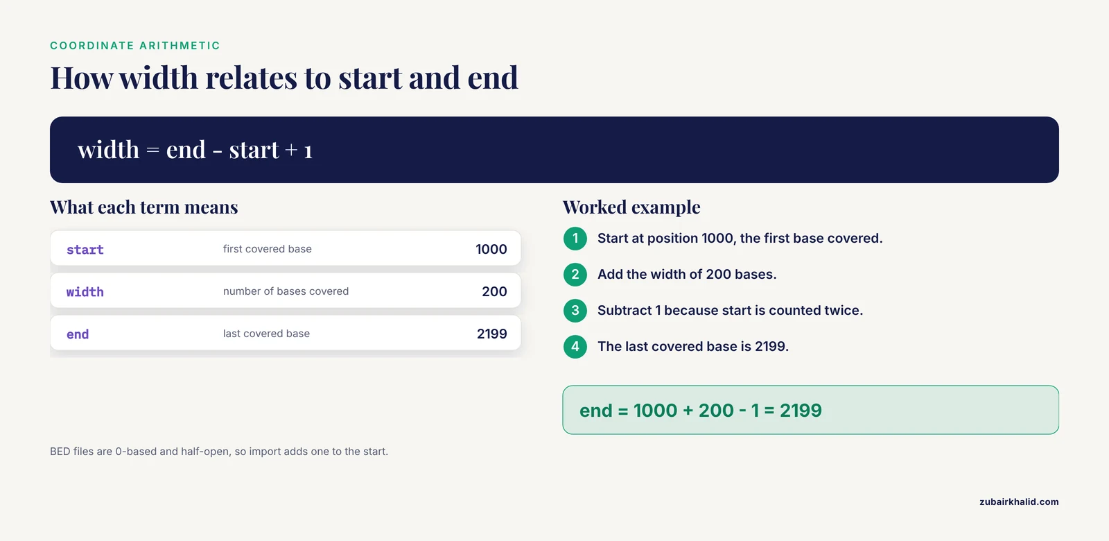
GRanges uses 1-based, closed intervals, matching the convention of most biological file formats and of R itself. A range with start 1000 and width 200 covers positions 1000 through 2199 inclusive, and width() equals end() - start() + 1. There is no half-open trickery at the class level. Coordinate conversion is a real source of confusion because file formats differ: BED files are 0-based, half-open, while GFF, GTF, VCF, and BAM are 1-based, and import tools handle the shift for you. We return to this in the mistakes section.
Building a GRanges: A Short Bioconductor Tutorial
Nothing teaches the structure faster than constructing one. Open an R session and run the following.
library(BiocManager)
BiocManager::install("GenomicRanges")
library(GenomicRanges)

gr <- GRanges(
  seqnames = c("chr1", "chr1", "chr2"),
  ranges   = IRanges(start = c(1000, 2500, 500),
                     width = c(200, 100, 300)),
  strand   = c("+", "-", "*"),
  score    = c(12.5, 8.1, 3.3),
  peak_id  = c("pk_1", "pk_2", "pk_3")
)

gr
Printing the object shows three header lines (seqnames, ranges, strand) followed by the metadata columns score and peak_id. Now inspect the pieces:
length(gr)          # 3
width(gr)           # 200 100 300
seqnames(gr)        # factor-like vector of chromosome names
mcols(gr)           # the DataFrame of metadata columns
seqinfo(gr)         # empty lengths until you fill them in
Fill in the genome context, which you should treat as part of object construction rather than an afterthought:
seqinfo(gr) <- Seqinfo(seqnames = c("chr1", "chr2"),
                       seqlengths = c(248956422, 242193529),
                       genome = "hg38")
Those lengths are the GRCh38 chromosome 1 and 2 sizes. From this point, trim() knows where the chromosome ends, and any object you compare against gr will advertise whether it uses the same assembly. Subsetting and column access behave as you would hope:
gr[gr$score > 5]        # keep only high-scoring intervals
gr$peak_id              # extract one metadata column
sort(gr)                # order by seqnames then strand then range
For nested structures, such as all exons grouped by gene, the companion class GRangesList holds one GRanges per list element. Many functions in the package operate on either form, and unlist() flattens a GRangesList into a single GRanges while split() rebuilds the grouping. When you eventually work with experiment-scale containers, the same pattern continues upward: a SummarizedExperiment stores row ranges and column data alongside an assay matrix, and packages like tidyCoverage build directly on that foundation to compare coverage tracks across thousands of genomic loci [6].
Core Operations, Step by Step
The GenomicRanges package earns its place in R for bioinformatics through interval algebra. The operations fall into four families.
1. Shifting and Reshaping Individual Ranges
These functions return a new GRanges of the same length and never modify the input, because S4 objects in Bioconductor follow copy-on-modify semantics.
shift(gr, 100)                          # move every range 100 bp to the right
resize(gr, width = 50, fix = "start")   # keep the start, take 50 bp
resize(gr, width = 50, fix = "center")  # keep the center
flank(gr, width = 100)                  # 100 bp upstream of each range
promoters(gr, upstream = 2000, downstream = 200)  # standard promoter window
resize() respects strand by default: fix = "start" anchors the 5-prime end, which is the transcript start on a minus-strand feature. Pass ignore.strand = TRUE when you want purely coordinate-based behavior.
2. Set Operations Within One Object
reduce() merges overlapping and abutting ranges into disjoint intervals, collapsing duplicates. disjoin() breaks ranges at every boundary so each output interval is covered by the same set of inputs throughout. range() gives the span from each group's minimum start to maximum end, gaps and all. These are the workhorses for turning raw peak calls or alignment blocks into clean, non-redundant feature sets.
3. Set Operations Between Two Objects
union(), intersect(), setdiff(), and gaps() combine two GRanges. A subtle point that trips up newcomers: for a first argument with multiple strands or chromosomes, these functions operate per strand and per chromosome, so union() of a plus-strand range and a minus-strand range at identical coordinates returns two rows, not one. union(x, ignore.strand = TRUE) does what most people expect when strand is irrelevant.
4. Overlaps, the Single Most Used Family
hits <- findOverlaps(query = peaks, subject = promoters_gr)
countOverlaps(promoters_gr, peaks)      # how many peaks per promoter
nearest(peaks, genes_gr)                # closest feature to each peak
findOverlaps() returns a Hits object with query and subject indices, and subjectHits(hits) pulls the matching rows of the subject. Overlap means any shared base by default; a minimum overlap width can be requested with minoverlap. Again, strand is honored by default and ignore.strand = TRUE disables that.
How GRanges Fits Inside a Real Workflow
A concrete walk-through shows why the class is described as infrastructure rather than a tool. A typical ChIP-seq or ATAC-seq analysis in the Bioconductor environment proceeds as follows:
- Read sequencing reads with ShortRead, an R/Bioconductor package for "input, quality assessment and exploration of high-throughput sequence data" that connects the read files to the rest of the R ecosystem [7].
- Align reads with an external aligner and import the resulting BAM file. The alignments arrive as a GRanges (or a close relative, a GAlignments object), one range per alignment.
- Call peaks with an external peak caller and import the peak coordinates. They are now a GRanges with a score metadata column.
- Use
reduce()to merge overlapping peaks across replicates,findOverlaps()to assign peaks to promoters, andcountOverlaps()to build a count matrix for differential binding analysis. - Export the final intervals back to BED or bigBed for genome browser viewing, or hand them to a visualization package. chromPlot accepts GRanges-format input and draws multiple tracks of regions, histograms, and continuous values along whole chromosomes, which makes processing errors visible that a table view would hide [5].
The same shape repeats across data types. TFBSTools scans whole genomes with transcription factor position weight matrices and reports binding sites as coordinate-bearing results, fitting directly into interval-based downstream analysis such as overlap with open chromatin [8]. CAGEr works with cap analysis gene expression data at single base-pair resolution, producing precise transcription start sites whose value comes from exact coordinate arithmetic, adding bases to find shifted TSSs and merging promoter clusters [9]. Chromatin interaction data extend the idea from one interval to a pair of intervals. GenomicInteractions was built for manipulating and investigating chromatin interaction data from Hi-C and ChIA-PET, with annotation and summarization at the level of individual interactions and of sets of genomic features [2], and InteractionSet generalizes that container so any two-dimensional genomic relationship can be stored and processed with the same conventions [1].
The most recent development keeps the same container but changes the grammar around it. The tidyomics ecosystem bridges Bioconductor objects, including GRanges, to the tidy R paradigm, letting analysts chain interval operations with dplyr-style verbs across six data frameworks and ten tools, demonstrated on 7.5 million cells from the Human Cell Atlas [10]. For an analyst coming to R from the tidyverse, this means the underlying structure stays constant while the interface becomes familiar.
GRanges Compared With the Objects It Gets Confused With
| Object | What it is | Key difference from GRanges |
|---|---|---|
| GRanges | S4 class for stranded genomic intervals with metadata | The thing itself. Lives in the GenomicRanges package. |
| GenomicRanges | Bioconductor package | A package cannot be subsetted or overlapped. It provides GRanges. |
| IRanges | S4 class for integer intervals | No chromosome, no strand, no seqinfo. The parent of the ranges slot. |
| GRangesList | List of GRanges, one element per group (for example per gene) | Nested structure. unlist() and split() convert in both directions. |
| data.frame or tibble | Generic table | Columns are not coordinate-validated, no strand semantics, no overlap algebra, no genome metadata. |
| SummarizedExperiment | Experiment container with rowRanges, colData, and assays | Wraps a GRanges in the rowRanges slot and adds a sample-by-feature matrix. |
| GAlignments | Aligned reads container (GenomicAlignments package) | Adds CIGAR strings and mapping information on top of interval logic. |
Import and Export in Practice
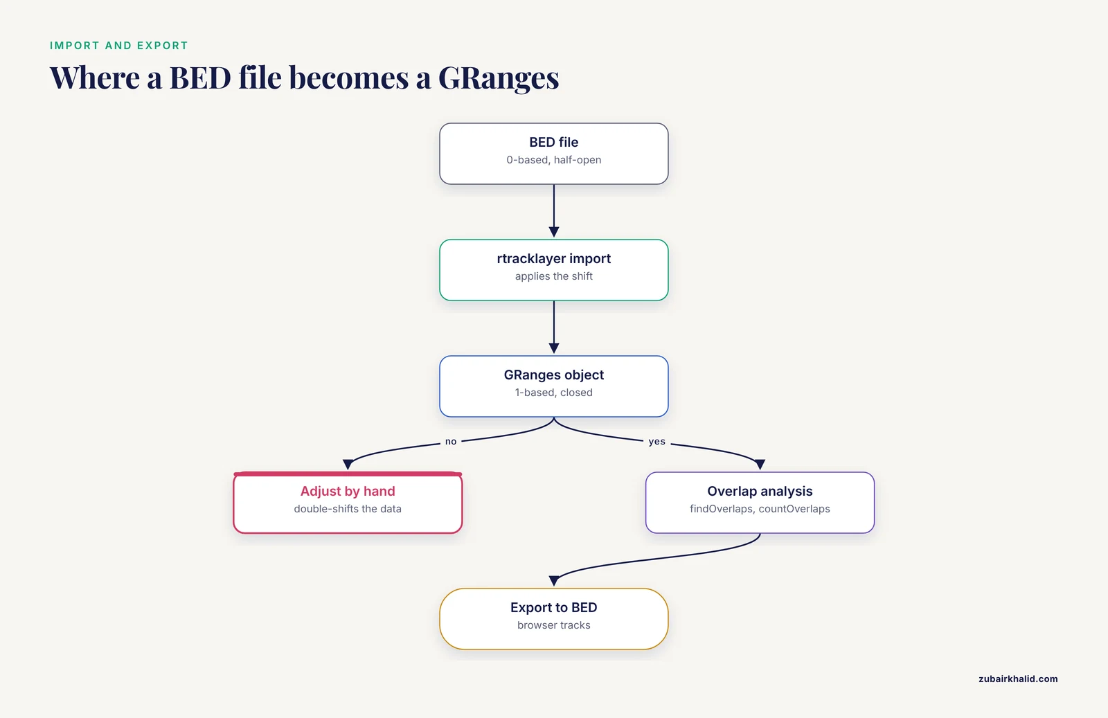
Almost no one types coordinates by hand after the tutorial stage. The usual entry points are file imports that produce GRanges directly:
- BED, GFF, GTF, bigBed, bigWig via the rtracklayer package, whose
import()andexport()functions handle the coordinate convention of each format. - VCF via the VariantAnnotation package, where each variant occupies one row and the INFO and FORMAT fields become metadata columns.
- BAM via Rsamtools or readGAlignments, then
as(..., "GRanges")to drop to plain intervals. - Peaks from MACS2 or similar callers, typically narrowPeak BED files, imported as GRanges with score and signal columns.
The reverse trip matters just as much, because collaborators and reviewers want browser tracks. export() writes GRanges back to any supported format, and packages such as chromPlot let you go straight from in-memory GRanges to chromosome-level figures without intermediate files [5]. As a rule for reproducible work, record the genome build and the import path in a script, not in your memory. Bioconductor packages ship vignettes that document these workflows, and the ShortRead paper describes the vignette tradition, outlining typical work flows inside the package itself, a convention the whole project follows [7].
Verifying and Debugging a GRanges Object
Because GRanges is an S4 class with validity rules, several checks catch problems early:
class(gr)confirms what you actually hold. Objects that look like GRanges but are data frames with chromosome columns will fail silently in overlap functions.validObject(gr)runs the formal validity checks.sum(width(gr))gives total covered bases, a fast sanity number when merging intervals.seqinfo(gr)compared between two objects reveals assembly mismatches before an overlap call silently returns empty results.table(strand(gr))exposes accidental strand pollution, a common artifact when concatenating datasets where one source was unstranded.sessionInfo()in the analysis record pins package versions, which is the standard Bioconductor reproducibility practice.
Common Mistakes and Limitations
Confusing the package with the class. The most frequent error behind searches for granges vs genomicranges is calling GenomicRanges() as a function. There is no such constructor. The constructor is GRanges(), and the package is only the container that ships it. Reading ?GRanges after library(GenomicRanges) resolves most of these errors.
Off-by-one errors from mixed file formats. BED is 0-based and half-open. Every GRanges operation assumes 1-based and closed. If a variant at BED position 100 appears at position 101 after import, that is the format conversion working correctly, not a bug. The error appears when people manually add or subtract one to fix a perceived problem and thereby double-shift their data. Trust the import function and check a few known loci instead.
Ignoring strand semantics. Three failure patterns recur. Assuming *-strand ranges will never match stranded features when they are the ones being queried in the wrong direction. Using resize() with fix = "start" on minus-strand features and getting downstream windows instead of upstream ones. And running findOverlaps() without thinking about whether the biology is strand-specific. Each has a one-argument fix, but only if you notice the problem.
Treating a GRanges like a tidy table. You can run as.data.frame(gr), and sometimes you should, but converting back and forth loses the coordinate validation and strand-aware operations that justify the class in the first place. A better path for tidy-minded analysts is the plyranges-style interface within the tidyomics ecosystem, which applies tidy grammar directly to genomic objects [10].
Empty or stale seqinfo. A GRanges built from a BED file often has chromosome lengths of NA. Overlaps still work, but trim() cannot clip, boundary checks fail, and assembly mismatches go undetected. Populate seqlengths from a known annotation source as part of the import step.
Zero-width expectations. Some analysts want zero-width ranges to mark point events. GRanges forbids them. Use width 1 and document the convention in your code.
Memory limits. GRanges holds everything in memory. For most peak, variant, and gene sets this is fine. For extremely large interval collections, the design question resembles the one beachmat addresses for matrices, where the choice among dense, sparse, and file-backed representations involves an explicit memory and speed trade-off [3]. Know the approximate row count and column burden of your object before scaling a pipeline.
Assuming all packages accept every GRanges flavor. Some functions expect unstranded input, some expect a GRangesList, and some expect specific metadata column names. Reading the function documentation for the expected input class is faster than debugging a cryptic error.
Quick Review
- GenomicRanges is the Bioconductor package. GRanges is the S4 class it defines. The class name is plural because one object holds many intervals.
- Every GRanges stores three parallel vectors: seqnames, an IRanges object with start and width, and strand with levels
+,-, and*. - Metadata columns travel inside the object via mcols and move with their ranges through every subset and overlap operation.
- seqinfo records chromosome lengths and the genome build, enabling trimming and mismatch detection.
- Coordinates are 1-based and closed. Width equals end minus start plus one. BED files are 0-based and half-open, and import functions handle the conversion.
- Core families of operations: reshape (shift, resize, flank, promoters), intra-object set algebra (reduce, disjoin), inter-object set algebra (union, intersect, setdiff), and overlaps (findOverlaps, countOverlaps, nearest).
- GRangesList nests intervals per group. SummarizedExperiment and its descendants build experiment matrices on top of the same row-range concept, which is how packages from GenomicInteractions [2] to tidyCoverage [6] stay interoperable.
Frequently Asked Questions
What does GRanges vs GenomicRanges mean?
GenomicRanges is the Bioconductor package and GRanges is the interval-holding class defined inside it. When someone says they loaded GenomicRanges, they loaded the library. When they say they have a GRanges, they hold an object of intervals with metadata.
Is a GRanges just a data frame?
No. It is an S4 object with validated, parallel components and attached genome metadata. It prints like a table and supports $ access, but its value lies in strand-aware, coordinate-validated interval algebra that data frames do not provide.
How do I get a BED file into a GRanges?
Use rtracklayer::import("file.bed"), which returns a GRanges with the BED score and name columns as metadata. The function applies the 0-based to 1-based coordinate conversion, so never adjust coordinates by hand afterward.
What is the difference between GRanges and GRangesList?
A GRanges is one flat collection of intervals. A GRangesList is a list of GRanges objects, typically one element per gene or per transcript, and it is the standard shape for exon-level annotations. Use unlist() to flatten and split() to regroup.
Why did my coordinates shift after importing a BED file?
They shifted once, correctly. BED is 0-based and half-open while GRanges is 1-based and closed, so import adds one to the start. The apparent shift is the file format convention, and re-shifting by hand will put your data one base off.
Do I need GenomicRanges before trying tidy-style genomics tools?
Yes, at least conceptually. Tidy interfaces in the tidyomics ecosystem operate on the same Bioconductor objects and inherit their coordinate and strand semantics [10]. Understanding the GRanges structure underneath makes the tidy wrappers predictable rather than magical.
Sources
- Infrastructure for genomic interactions: Bioconductor classes for Hi-C, ChIA-PET and related experiments.
- GenomicInteractions: An R/Bioconductor package for manipulating and investigating chromatin interaction data.
- beachmat: A Bioconductor C++ API for accessing high-throughput biological data from a variety of R matrix types.
- Orchestrating multi-state QTL analysis with Bioconductor.
- chromPlot: visualization of genomic data in chromosomal context.
- Epigenomics coverage data extraction and aggregation in R with tidyCoverage.
- ShortRead: a bioconductor package for input, quality assessment and exploration of high-throughput sequence data.
- TFBSTools: an R/bioconductor package for transcription factor binding site analysis.
- CAGEr: precise TSS data retrieval and high-resolution promoterome mining for integrative analyses.
- The tidyomics ecosystem: enhancing omic data analyses.