How to Visualize Synteny and Phylogenetic Data Together with ggtree
By Dr. Zubair Khalid, DVM, MS, PhD ·

By the end of this article you will be able to build a single publication-ready figure in R that shows a phylogenetic tree with synteny blocks (conserved gene or sequence blocks, in their order along each genome) drawn alongside every tip. You will also be able to annotate the tree with clade shading, support values, and per-genome feature heatmaps, then export the result as a PDF or PNG at journal resolution.
To follow along you need R 4.2 or newer, the Bioconductor packages ggtree, treeio, ggtreeExtra, ggplot2, and ape, a rooted or unrooted tree in Newick format, and a table of synteny blocks with a genome name, a block identifier, a start coordinate, an end coordinate, and a strand or class label. Everything below runs in the R console or an R Markdown notebook and uses the ggplot2 grammar of graphics, which is the standard approach for R for bioinformatics plotting work.
Why Put Synteny and a Tree in One Figure
A phylogenetic tree tells you who is related to whom. A synteny map tells you how each genome is organized internally. When reviewers and readers see both in one figure, they can judge at a glance whether structural changes in the genomes follow the evolutionary relationships in the tree. This combined presentation has become a standard pattern in comparative genomics papers.
Recent studies show the pattern in action. A chloroplast genome study of Rosa platyacantha sequenced, assembled, and annotated the first complete plastid genome for that species and then ran comparative genomics and phylogenetic analyses against other Rosa chloroplast genomes, reporting a 157,133 bp genome with 132 genes and a GC content of 37.21% [1]. A mitochondrial genome study of Rhododendron simsii var. putuoense explicitly combined phylogenetic and synteny analyses and reported six homologous segments, covering 0.91% of the mitochondrial genome, as evidence of interorganellar gene transfer [2]. A study of the Korean endemic Arabis takesimana compared 32 Brassicaceae mitogenomes and found that 30 protein-coding genes were conserved across sampled taxa while others showed lineage-specific truncation, pseudogenization, or loss [3]. In bacteria, a genus-wide analysis of 1,740 Pseudomonas genomes mapped the patchy distribution of LuxI/R quorum sensing systems and LuxR solo regulators onto phylogeny to distinguish vertical inheritance from horizontal transfer [4].
All of these papers needed the same core figure: a tree, plus per-genome structural tracks. The ggtree package, maintained in the Bioconductor project, is the most widely used R tool for that job. This article is a Bioconductor tutorial style walkthrough of that exact workflow.
The Core Pattern of ggtree Synteny Phylogenetic Visualization
The mental model is simple. ggtree converts a tree into a fortified data frame where every node and tip has an x position (relatedness or depth) and a y position (vertical order). Any ordinary ggplot2 layer can then be drawn against those coordinates. Synteny blocks are just rectangles or segments positioned in a small per-genome coordinate system. You attach them to the tip positions with one of three tools:
geom_fruit()from ggtreeExtra, which draws an independent data panel around a circular or fan tree.facet_plot()from ggtree, which adds a faceted panel to a rectangular tree.msaplot()from ggtree, which draws a multiple sequence alignment next to the tree, useful when your synteny evidence is a locus-level alignment.
Upstream tools still matter. ggtree does not detect synteny. You produce the block table with Mauve, MCScanX, progressiveMauve, BLAST-based collinearity scripts, or ortholog grouping, then hand the tidy result to ggtree. This separation is a feature because you control what counts as a homologous block.
Step-by-Step Walkthrough
The following ggtree synteny phylogenetic visualization step by step walkthrough uses a small toy dataset so you can verify every intermediate result. Six genomes, six blocks each. When you switch to your own data, only the tree file and the block table change.
Step 1: Install and Load the Packages
if (!require("BiocManager", quietly = TRUE)) {
  install.packages("BiocManager")
}
BiocManager::install(c(
  "ggtree", "treeio", "ggtreeExtra", "ggplot2", "ape", "ggnewscale"
))

library(treeio)      # reading and writing tree files
library(ggtree)      # tree visualization
library(ggtreeExtra) # outer data layers via geom_fruit
library(ggplot2)     # layers, scales, themes
library(ape)         # read.tree and tree utilities
BiocManager is the standard installer for Bioconductor packages. ggtree, treeio, and ggtreeExtra live on Bioconductor, so CRAN's install.packages("ggtree") alone is not enough on a fresh machine.
Step 2: Read the Tree
tree <- read.tree(text = paste0(
  "(((GenomeA:0.032,GenomeB:0.028):0.041,",
  "(GenomeC:0.025,GenomeD:0.021):0.018):0.030,",
  "(GenomeE:0.040,GenomeF:0.044):0.035);"
))
tree$tip.label
Expected output:
[1] "GenomeA" "GenomeB" "GenomeC" "GenomeD" "GenomeE" "GenomeF"In real work the Newick string comes from a tree builder. Alignment-based tree builders such as IQ-TREE or RAxML output Newick directly. Genome-scale trees can also come from distance methods, for example average nucleotide identity (ANI) and digital DNA-DNA hybridization, which is how a recent Rahnella study established that its polar isolate formed a distinct genomic lineage within the genus [5]. Confirm the tips before plotting:
length(tree$tip.label)   # 6
is.binary(tree)          # TRUE for most builder output
Step 3: Build the Synteny Block Table
ggtree wants tidy data, one row per block per genome. Build your table with a script from whichever upstream tool you ran. For the demo, construct it directly:
blocks <- list(
  GenomeA = c(1, 14, 30, 42, 55, 70),
  GenomeB = c(2, 15, 28, 40, 57, 68),
  GenomeC = c(1, 16, 31, 41, 54, 72),
  GenomeD = c(2, 13, 30, 43, 56, 71),
  GenomeE = c(1, 15, 29, 41, 55, 70),
  GenomeF = c(3, 14, 27, 44, 58, 69)
)
widths <- c(10, 11, 9, 12, 10, 8)
strand <- c(1, 1, -1, 1, -1, 1)
class  <- c("conserved", "conserved", "inverted",
            "conserved", "translocated", "conserved")

synteny <- do.call(rbind, lapply(names(blocks), function(g) {
  data.frame(
    tip   = g,
    block = seq_along(blocks[[g]]),
    start = blocks[[g]],
    end   = blocks[[g]] + widths,
    strand = strand,
    class = class,
    stringsAsFactors = FALSE
  )
}))
head(synteny)
Expected output:
       tip block start end strand      class
1 GenomeA     1     1  11      1  conserved
2 GenomeA     2    14  25      1  conserved
3 GenomeA     3    30  39     -1   inverted
4 GenomeA     4    42  54      1  conserved
5 GenomeA     5    55  65     -1 translocated
6 GenomeA     6    70  78      1  conserved
In a real project, columns map to real quantities. If you work with plant organellar genomes, the start and end columns might come from a Mauve backbone file in base pairs, and the class column might encode inversions or translocations. The Rhododendron mitogenome study is a good model of what these tables look like in practice, because it reported homologous segments between mitochondrial and plastid genomes with defined coordinates spanning 0.91% of the mitochondrial genome [2].
Step 4: Compute Tip Positions
Both geom_fruit() and facet_plot() need the internal y coordinate that ggtree assigns to each tip. Extract it once and merge it into your block table:
td <- ggtree(tree)$data
synteny$y <- td$y[match(synteny$tip, td$label)]
stopifnot(!any(is.na(synteny$y)))
The stopifnot() line is your first validation check. If any y came back as NA, a tip label in the block table does not match the tree exactly.
Step 5: Draw the Tree
p <- ggtree(tree, layout = "fan", open.angle = 20, size = 0.7) +
  geom_tippoint(size = 1.6)
p
Parameters that matter here:
layout = "fan"arranges tips radially, leaving room for outer panels."rectangular"is the alternative when you preferfacet_plot().open.angle = 20leaves a 20 degree gap in the circle so tip labels are not cut where the circle closes.sizecontrols branch line width. Keep it between 0.5 and 1.0 so annotations dominate the figure, not the branches.
Step 6: Add the Synteny Panel with geom_fruit
p1 <- p +
  geom_fruit(
    data = synteny,
    geom = geom_segment,
    mapping = aes(
      x     = start,
      xend  = end,
      y     = y,
      yend  = y,
      color = class
    ),
    linewidth = 3,
    offset = 0.5,
    pwidth = 0.8
  ) +
  scale_color_manual(
    values = c(
      conserved    = "#2C7FB8",
      inverted     = "#D95F02",
      translocated = "#66A61E"
    )
  )
p1
Reading the parameters:
datais your tidy block table, now carrying theycolumn.geommust be the function object itself,geom_segment, not a call such asgeom_segment(). Passing the called object is a frequent source of add-layer errors.mappingplaces each block fromstarttoendat the tip'syposition. Becauseyend = y, each block renders as a short horizontal segment.offsetpushes the panel away from the tree tips andpwidthsets the radial thickness the panel occupies. Both are scaled against the tree depth, so with shallow trees use small values and adjust by eye.linewidthis the segment thickness. With three or more blocks stacked per tip throughposition_dodge(), reduce it.
Because each fruit panel has its own independent x scale, the coordinate units of your blocks (base pairs, kilobases, or block indices) do not need to match the tree's branch length scale. That independence is what makes geom_fruit() the workhorse for ggtree synteny phylogenetic visualization.
To add a second fruit panel, for example repeat density, just chain another geom_fruit() with a larger offset.
Step 7: Annotate Clades and Support Values
Internal node numbers are invisible until you print them. A quick diagnostic plot reveals them:
ggtree(tree) +
  geom_text2(aes(subset = !isTip, label = label), hjust = -0.3, size = 2.2)
label on internal nodes holds whatever the tree builder wrote there, which for IQ-TREE or RAxML output is usually ultrafast bootstrap support or SH-aLRT values. Once you know the node number of the clade you care about, shade and label it:
p2 <- p1 +
  geom_hilight(node = 10, fill = "#CBD5E1", alpha = 0.4) +
  geom_cladelabel(
    node = 10,
    label = "Clade I",
    offset = 1.2,
    barsize = 1.5,
    color = "#334155"
  )
This is exactly the layer used when studies annotate haplogroups on mitochondrial trees. The barn swallow phylogeographic analysis, which screened 580 complete Hirundo rustica mitochondrial genomes plus twelve related species, defined five major haplogroups including a novel haplogroup E, and such haplogroup assignments are typically drawn as clade labels or shaded clades on the tree [6].
Step 8: Add a Feature Heatmap Track
Trees and synteny answer structure questions. Numeric genome features belong in a strip heatmap beside the tree via gheatmap():
feat <- data.frame(
  PCGs    = c(34, 34, 33, 33, 34, 34),
  repeats = c(21, 19, 24, 22, 20, 20)
)
rownames(feat) <- tips

p3 <- gheatmap(p2, feat, offset = 2.5, width = 0.25,
               colnames = FALSE, color = NA) +
  scale_fill_viridis_d()
rownames(feat) must match tip labels exactly. Because the heatmap uses the fill aesthetic while your synteny panel uses color, the two scales coexist. If you need a second fill scale, load ggnewscale and call new_scale_fill() between layers.
This pattern generalizes to any per-genome count or binary annotation. A moss mitochondrial genome study, for instance, reported 189 RNA editing sites in the mitochondrial genome and 608 in the chloroplast genome of Rhodobryum laxelimbatum, the kind of per-genome counts that map naturally onto heatmap tracks [7]. The Arabis takesimana study reported mitogenome features such as 21.83 kb of transposable element sequence and 44.03 kb of repetitive DNA, and found a strong positive association between mitogenome size and TE content across 32 Brassicaceae mitogenomes, a result you would visualize exactly this way [3].
Step 9: The Rectangular Alternative with facet_plot
For a linear layout, facet_plot() is often easier because it manages its own panel and joins data to tips by the first column:
pr <- ggtree(tree) +
  geom_tiplab(size = 2.8, hjust = -0.1)

facet_plot(
  pr,
  panel = "Synteny",
  data = synteny,
  geom = geom_segment,
  mapping = aes(
    x = start, xend = end,
    y = y, yend = y,
    color = class
  ),
  linewidth = 3
)
facet_plot() looks up the y values itself when the first column of data holds tip labels, so here the explicit y merge from Step 4 is redundant but harmless. The panel argument names the new facet column, which ggplot2 renders to the right of the tree with its own x axis.
Step 10: Locus-Level Synteny with msaplot
When your structural evidence is a set of aligned loci rather than genome-scale blocks, msaplot() draws the alignment beside the tree:
p_msa <- msaplot(p, fasta = "locus_alignment.fasta",
                 offset = 0.6, width = 2)
Each row of the alignment hangs off its tip, so shared sequence organization across the alignment reads as fine-scale synteny. This suits cases where a single conserved region carries the biological signal, such as the mitochondrial plastid DNA insertion reported in Arabis takesimana, which contributed four intact plastid-derived tRNA genes and a partial rrn18 segment into the mitogenome [3].
Step 11: Save and Verify
ggsave("tree_synteny.pdf", p3, width = 10, height = 10, useDingbats = FALSE)
ggsave("tree_synteny.png", p3, width = 10, height = 10, dpi = 300)
Three checks before you call it done:
- Every tip has the expected number of blocks.
table(synteny$tip)should show six rows per genome in the demo, or your known block count in real data. - Nothing matches a tree tip that should not exist.
setdiff(synteny$tip, tree$tip.label)must returncharacter(0). - The panel visually aligns with the tips. Temporarily enlarge
geom_tippoint()and confirm each block row sits level with its tip point, then shrink the points back.
Reference Table of Key Functions
| Function | Package | Purpose | Arguments that matter |
|---|---|---|---|
| , - | , - | , - | , - |
ggtree() | ggtree | Base tree layer | layout, open.angle, size |
geom_fruit() | ggtreeExtra | Independent outer data panel, ideal for circular trees | data, geom, mapping, offset, pwidth |
facet_plot() | ggtree | Faceted data panel for rectangular trees, joins by first column | panel, data, geom, mapping |
gheatmap() | ggtree | Heatmap strip of per-tip numeric or categorical features | data, offset, width, colnames |
msaplot() | ggtree | Multiple sequence alignment drawn beside the tree | fasta, offset, width |
geom_tiplab() | ggtree | Tip labels | size, offset, hjust |
geom_hilight() | ggtree | Clade background shading | node, fill, alpha |
geom_cladelabel() | ggtree | Clade label with a connecting bar | node, label, offset, barsize |
geom_text2() | ggtree | Text on internal nodes, used for support values | subset, label |
hexpand() | ggtree | Extra horizontal room in rectangular layouts | ratio |
Common Mistakes and Limitations
Assuming tree tips and table labels match silently. The most frequent failure in ggtree synteny phylogenetic visualization is a label mismatch. One trailing space, one underscores-versus-spaces difference, and the fruit panel quietly drops rows or errors out. Run setdiff() in both directions and fix labels at the source, ideally by regenerating the Newick from the same annotation file that produced the block table.
Passing a called geom instead of the geom function. In geom_fruit(), the geom argument takes the function itself. Write geom = geom_segment, not geom = geom_segment(). The called version makes ggplot2 throw an add-layer error because it receives a complete layer object where a geometry constructor is expected.
Forgetting that geom_fruit() lives in ggtreeExtra. If you load only ggtree and call geom_fruit(), R reports Error: could not find function "geom_fruit". Install and attach ggtreeExtra.
Missing the internal y column. geom_fruit() needs y mapped for the fruit layer to find the tips. Without it you get an aesthetic-mapping error such as object 'y' not found. Compute y from ggtree(tree)$data and merge it in, as in Step 4.
Mixing scales across layers. gheatmap uses fill, fruit layers often use color or fill. Two layers claiming fill produce the ggplot2 message Scale for fill is already present. Insert ggnewscale::new_scale_fill() between the layers or consolidate aesthetics.
Reading synteny panels as whole-genome collinearity. A block table shows where conserved or homologous segments sit, not that two genomes are fully collinear. The Rhododendron study is a good calibration point, since its six interorganellar homologous segments covered less than one percent of the mitogenome even though the figure communicates real transfer events [2]. Label panels with their true scope.
Coloring SNP-threshold clusters as if they were clades. When annotating bacterial trees, be careful with transmission or outbreak clusters defined by a pairwise SNP distance cutoff. A study of tuberculosis datasets in the United Kingdom and Thailand found that low-threshold SNP clustering often produced non-monophyletic clusters, and that consistency with tree-based clustering required thresholds of at least 22 SNPs in the Thai data [8]. Before you shade a cluster with geom_hilight(), verify monophyly, or your figure will assert a clade the tree contradicts.
Overplotting with too many blocks or tips. Dozens of fine blocks per tip turn the panel into noise. Aggregate small blocks, facet by class, or split genomes across figure panels. Studies built on very large datasets, such as the 580-mitogenome swallow analysis [6], routinely present the full tree separately from structural detail for this reason.
Expecting ggtree to interpret your biology. ggtree draws what you hand it. Deciding which segments count as syntenic, which clade deserves shading, and which genes are orthologous is your responsibility and comes from upstream analyses such as those in the comparative studies cited above. Also remember that branch lengths and topologies depend on the marker set and method. A chloroplast genome phylogeny [1] and a genome-wide bacterial phylogeny [5] can legitimately differ in scale and resolution, so never transfer coordinates or support values between trees.
A Decision Framework: Which Panel Function Fits Your Data
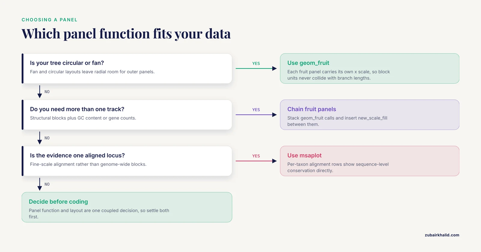
The original walkthrough introduces geom_fruit(), facet_plot(), gheatmap(), and msaplot() as tools, but it does not give you a rule for choosing between them before you start coding. That choice drives everything downstream: the tree layout, how you prepare the block table, and how many panels you can stack before the figure collapses into noise. Make the decision first with this table.
| Situation | Best tool | Why |
|---|---|---|
| - | - | - |
| Circular or fan tree, one structural track | geom_fruit() | Each fruit panel carries its own x scale, so block coordinates never collide with branch lengths |
| Circular or fan tree, two or more structural tracks | Chained geom_fruit() calls with ggnewscale | Panels stack radially, each with independent scales |
| Rectangular tree, one or two tracks | facet_plot() | The facet machinery gives you a labeled x axis for block coordinates, which circular layouts cannot show cleanly |
| Per-genome numeric features such as gene counts or editing sites | gheatmap() | One compact strip answers size and content questions without a full panel |
| Fine-scale alignment evidence at one locus | msaplot() | Per-taxon alignment rows show sequence-level conservation directly |
| Hundreds of tips | Facet split or separate figures | No single panel survives that density intact |
Three scenarios make the rule concrete.
Scenario one: you are comparing a dozen organellar genomes, as in the Rosa platyacantha chloroplast study, where the complete plastid genome of 157,133 bp with 132 genes and 37.21% GC content was compared against other Rosa plastomes [1]. At twelve tips, either layout works. If the paper figure needs block order legible for every genome, choose rectangular with facet_plot(), because you get a real x axis in kilobases that readers can read.
Scenario two: you are placing structural variants on a bacterial species tree with a hundred isolates, similar in spirit to the genus-wide Pseudomonas analysis that mapped quorum sensing gene distribution onto phylogeny across 1,740 genomes [4]. A fan layout with geom_fruit() wins, because radial space accommodates many tips and each accessory-gene track gets its own scale.
Scenario three: your key claim is that one specific region moved between genomes, like the mitochondrial plastid DNA insertion in Arabis takesimana that carried four intact plastid-derived tRNA genes and a partial rrn18 segment into the mitogenome [3]. Here msaplot() on that single locus is the honest figure, because the alignment itself is the evidence.
A frequent misconception is that geom_fruit() only works on circular trees. It is designed for them, and its offset and width parameters are tuned for radial layouts, but the deeper point is that the choice of panel function and the choice of layout are coupled decisions. Decide them together before writing any plotting code, and you avoid the most common mid-project refactoring.
From Upstream Tool Output to a Tidy Block Table
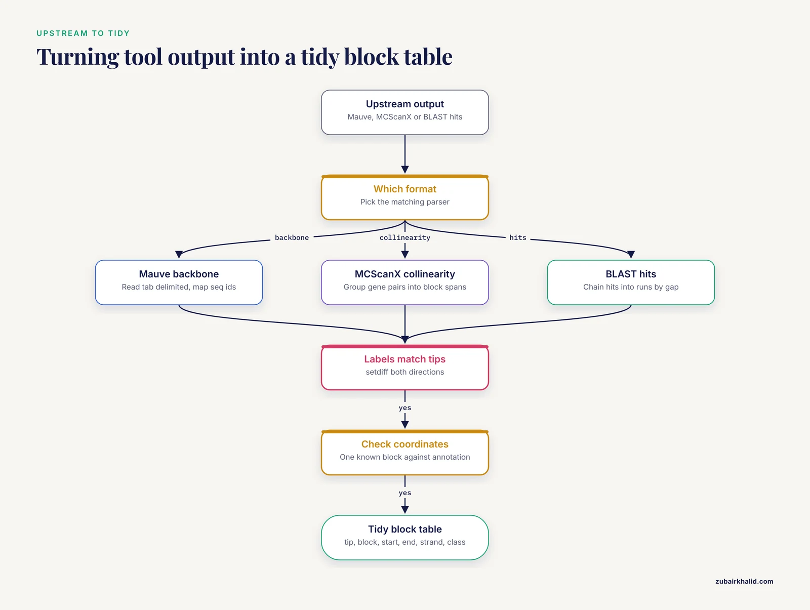
The toy table in the main walkthrough is hand-built. Real projects fail here, not in ggplot2. This section shows parsing patterns for the three most common upstream formats. Install the helpers first if they are missing:
install.packages(c("dplyr", "tidyr", "readr"))
library(dplyr)
library(tidyr)
library(readr)
Parsing a Mauve or progressiveMauve backbone file
Backbone files are tab delimited, with one row per block per genome sequence, columns for the sequence identifier, start and end coordinates, and orientation. The identifiers usually concatenate genome and contig names, which will not match your tree tips verbatim. Plan a mapping step:
backbone <- read_tsv("mauve_backbone.txt",
                     col_names = c("seq_id", "block", "start", "end", "strand"),
                     comment = "#")

# Map full sequence identifiers to tree tip labels
label_map <- c(
  "GenomeA_contig1" = "GenomeA",
  "GenomeB_contig1" = "GenomeB"
  # one row per genome in your project
)

blocks <- backbone %>%
  mutate(tip = unname(label_map[seq_id])) %>%
  filter(!is.na(tip)) %>%
  select(tip, block, start, end, strand)
The filter(!is.na(tip)) line is doing real work. It silently removes blocks from any sequence not in your map, which is exactly what you want when draft assemblies contain plasmids or unplaced contigs you deliberately excluded from the tree.
Parsing MCScanX collinearity output
MCScanX writes a .collinearity file with header lines starting with ## and data rows containing paired gene identifiers and block scores. If your synteny evidence is gene-level collinearity between genomes, collapse each block to its span:
collin <- read_tsv("i upstream.collinearity", comment = "#",
                   col_names = FALSE, show_col_types = FALSE)

# Collapse paired gene rows into one row per block per genome pair
blocks <- collin %>%
  group_by(X1) %>%                       # block identifier column
  summarise(
    first_gene = min(X3, X4),
    last_gene  = max(X3, X4),
    n_genes    = n()
  )
Adapt the column indices to your file. The important pattern is group_by() plus summarise(): many gene pairs reduce to one block with a coordinate span, and that span is what ggtree draws.
Parsing BLAST tabular output into blocks
BLAST-based collinearity scripts emit tabular hits. A pragmatic approach is to chain hits along each chromosome into runs, then treat each run as a block:
hits <- read_tsv("hits.tsv", col_names = c(
  "qseqid", "sseqid", "pident", "length",
  "qstart", "qend", "sstart", "send", "evalue"
))

blocks <- hits %>%
  filter(pident >= 90, length >= 300) %>%
  arrange(sseqid, sstart) %>%
  group_by(sseqid) %>%
  mutate(gap = sstart - lag(send, default = first(sstart)),
         new_block = gap > 5000) %>%
  mutate(block = cumsum(new_block)) %>%
  group_by(sseqid, block) %>%
  summarise(start = min(sstart), end = max(send), .groups = "drop")
The two cutoff values shown, 90 percent identity and 5,000 bases of maximum gap, are placeholders for demonstration. Choose and justify your own thresholds; the parsing structure is what transfers between projects.
Coordinate conventions and off-by-one errors
Three conventions exist in the wild: one-based inclusive coordinates, zero-based half-open intervals, and two-column formats where one column means "position" and the other means "length". Before plotting, verify your table on one known block against the genome annotation. A block that should cover a gene you can find in the annotation file is your ground truth. If you discover a half-open interval, convert once, upstream of the plot:
# Convert zero-based half-open to one-based inclusive
blocks <- blocks %>% mutate(start = start + 1)
Fixing this in the parser rather than in the plotting layer keeps one source of truth. Also normalize units deliberately: organellar genomes in base pairs are fine for facet panels, but large bacterial genomes read better in megabases:
blocks <- blocks %>% mutate(start = start / 1e6, end = end / 1e6)Rendering Strand and Direction in Synteny Panels
The main walkthrough draws every block as a plain segment with geom_segment(). That hides the single most interesting piece of comparative information: direction. Inversions and reversed blocks are the structural changes most studies highlight, so render strand explicitly.
The simplest upgrade is an arrow:
p1 <- p +
  geom_fruit(
    data = synteny,
    geom = geom_segment,
    mapping = aes(
      x = start, xend = end,
      y = y, yend = y,
      color = class
    ),
    arrow = grid::arrow(length = unit(2, "mm"),
                        type = "closed"),
    linewidth = 3, offset = 0.5, pwidth = 0.8
  )
Every block now points in its reading direction, so a viewer can spot a reversed block without consulting the legend.
For blocks with real vertical thickness, geom_rect() gives better control, because you set ymin and ymax explicitly:
synteny$ymin <- synteny$y - 0.25
synteny$ymax <- synteny$y + 0.25

p_rect <- p +
  geom_fruit(
    data = synteny,
    geom = geom_rect,
    mapping = aes(
      xmin = start, xmax = end,
      ymin = ymin, ymax = ymax,
      fill = class
    ),
    offset = 0.5, pwidth = 0.9
  ) +
  scale_fill_manual(values = c(
    conserved = "#2C7FB8", inverted = "#D95F02",
    translocated = "#66A61E"
  ))
With rectangles you can go further and draw each block as two halves, one for each orientation, so that an inversion reads as a color switch at the break point. The Rhododendron simsii var. putuoense mitochondrial study reported six homologous segments between the mitogenome and plastid genome, covering 0.91% of the mitochondrial genome, as evidence of interorganellar transfer [2]. A figure for that result is more persuasive when each transferred segment is drawn with a direction arrow and a distinct class label, because the reader can then trace where each segment landed.
One caution: strand is a property of your input data, not something ggtree infers. If your upstream tool reports orientation, carry it through the tidy table as a column, even if you do not map it immediately. Blocks without orientation information should be labeled as such in the figure caption rather than silently drawn in one direction.
Ragged Block Counts and Dodging Multiple Blocks per Tip
The toy dataset gives every genome exactly six blocks. Real data is ragged. One genome may carry thirty blocks while its closest relative carries eleven, and some tips may carry none at all. Three problems follow, each with a specific fix.
First, blocks at the same tip overlap. If a genome has multiple blocks in the same class at overlapping or adjacent coordinates, or you are plotting one row per gene rather than one row per block, dodge them vertically:
p_dodge <- p +
  geom_fruit(
    data = synteny,
    geom = geom_segment,
    mapping = aes(x = start, xend = end, y = y, yend = y, color = class),
    linewidth = 1.2,
    position = position_dodge(width = 0.6),
    offset = 0.5, pwidth = 0.8
  )
position_dodge() nudges same-position rows apart within each tip. Reduce linewidth as the number of dodged rows grows; the walkthrough already warns of this, and the practical rule is that dodged rows look best when the combined thickness of all rows at one tip stays under the space of one tip interval.
Second, tips with zero blocks disappear from the panel. That is correct behavior, but readers may interpret the gap as missing data rather than absence. Add an explicit zero row for such tips, or state the convention in the caption. Check counts directly:
table(synteny$tip)
tips_without_blocks <- setdiff(tree$tip.label, unique(synteny$tip))
tips_without_blocks
Third, class distributions differ wildly across genomes. In the Arabis takesimana Brassicaceae mitogenome comparison, most protein-coding genes were conserved across the 32 sampled taxa while others showed lineage-specific truncation, pseudogenization, or loss [3]. A per-genome structural track for that dataset naturally produces ragged class counts, and that raggedness is the finding. Do not normalize it away by dropping rare classes; instead, group them:
blocks <- blocks %>%
  mutate(
    class = case_when(
      strand < 0 ~ "inverted",
      class %in% c("truncated", "pseudogene", "lost") ~ "degraded",
      TRUE ~ "conserved"
    )
  )
Collapsing rare categories into a small set keeps the legend readable while preserving the signal that some lineages carry degraded copies. This mirrors what published comparative genomics figures do: they summarize rare events rather than giving each one a color.
Inside the Circular Coordinate System
Many ggtree frustrations trace back to not understanding what the internal data frame contains. Inspect it deliberately:
td <- ggtree(tree)$data
head(td)
names(td)
You will find at minimum x, y, branch, label, isTip, and for fan layouts angle. Three practical consequences follow.
First, the x scale is in branch-length units. In the demo tree, tip depths are around 0.03 to 0.1, so an offset of 0.5 is five to fifteen times the tree depth. That sounds enormous but is correct, because the fan layout stretches those units across the full radius. On a tree with tips at depth 1.0, the same offset of 0.5 sits much closer to the tips. There is no universal offset value; scale it against max(td$x):
tree_depth <- max(td$x[td$isTip])
my_offset  <- tree_depth * 0.15
my_pwidth  <- tree_depth * 0.25
This ratio-based approach is what makes a plotting script portable between a shallow toy tree and a real one.
Second, tip label placement on circular layouts needs geom_tiplab2(), which rotates labels along the radial direction:
p + geom_tiplab2(size = 2.5, offset = tree_depth * 0.05)Using plain geom_tiplab() on a fan tree produces labels that overlap the branches at the bottom of the circle.
Third, open.angle interacts with label space. A 20 degree opening, as used in the walkthrough, is usually enough for labels if the longest label is short. With long species names, increase the opening and reduce label size together rather than fighting the overlap with trial and error.
A diagnostic trick that saves hours: plot a pure coordinate skeleton with no data panels before adding anything.
p +
  geom_tippoint(size = 2) +
  geom_fruit(
    data = synteny, geom = geom_point,
    mapping = aes(x = start, y = y, color = class),
    size = 0.8, offset = my_offset, pwidth = my_pwidth
  )
Single points are cheap to position. Once every block start appears at the correct radius and angle, switch to segments or rectangles. This isolates layout errors from geometry errors, which is far faster than debugging a fully annotated figure.
Stacking Multiple Panels and Managing Multiple Scales
A single synteny panel is rarely the whole story. Real figures combine a structural track, a feature heatmap, and often a categorical annotation such as geographic origin. Each panel may want the fill aesthetic, and ggplot2 allows only one fill scale per plot unless you intervene.
The intervention is ggnewscale::new_scale_fill() placed between layers:
library(ggnewscale)

p_multi <- p +
  # Panel 1: synteny blocks, fill-based
  geom_fruit(
    data = synteny, geom = geom_rect,
    mapping = aes(xmin = start, xmax = end,
                  ymin = ymin, ymax = ymax, fill = class),
    offset = 0.4, pwidth = 0.9
  ) +
  scale_fill_manual(values = c(
    conserved = "#2C7FB8", inverted = "#D95F02",
    translocated = "#66A61E"
  )) +
  new_scale_fill() +
  # Panel 2: a second fruit layer with its own fill scale
  geom_fruit(
    data = gc_content, geom = geom_tile,
    mapping = aes(x = position, y = y, fill = gc_bin),
    offset = 1.4, pwidth = 0.5
  ) +
  scale_fill_manual(values = c(low = "#FEE0B6", high = "#542788")) +
  new_scale_fill() +
  # Panel 3: heatmap strip
  gheatmap(p_last_layer_placeholder, feat, offset = 2.2, width = 0.25) +
  scale_fill_viridis_d()
Read the ordering rule carefully: new_scale_fill() must come after the scale it resets and before the layer that uses the new scale. A common failure is stacking two geom_fruit() calls with no new_scale_fill() between them and then receiving the "Scale for fill is already present" message, which the main walkthrough already flags; this section shows the structural fix rather than just the symptom.
A second ordering rule concerns legends. With multiple panels, ggplot2 collects all legends at the plot edge by default, and readers cannot tell which legend belongs to which panel. Fix this by naming the aesthetics descriptively:
labs(fill = "Block class") # set per scale with the `name` argumentand, when the figure still reads ambiguously, place each panel's legend via guides() with explicit titles such as "Block class", "GC content", and "Genome features". Every published figure combining these tracks, including the organellar genome studies cited throughout this article, has had to solve the same legend attribution problem, and explicit aesthetic names are the robust solution.
A third practical note: each additional fruit layer increases the total radial footprint. Budget it. Tree depth plus every offset plus every pwidth must fit inside the exported canvas. If your outermost panel clips in the PDF, either shrink earlier pwidth values or increase the export dimensions. Exporting at equal width and height for circular figures, as the export guidance recommends, keeps the radial geometry undistorted.
Reading Tree Builder Output Correctly
The walkthrough reads a Newick string with ape::read.tree(). That works, but it discards information that builder-specific files carry, and losing it creates avoidable work in the annotation step. treeio provides parsers for common builder output formats, and they preserve support statistics as separate data columns:
# IQ-TREE .treefile with SH-aLRT support and ultrafast bootstrap
tree_iq <- treeio::read.iqtree("alignment.treefile")

# RAxML best tree with bootstrap support
tree_rax <- treeio::read.raxml("RAxML_bipartitionsBranchLabels.run")

p_iq <- ggtree(tree_iq) +
  geom_tippoint(size = 1.6) +
  geom_text2(aes(subset = !isTip,
                 label = paste0(SH_aLRT, "/", UFboot)),
             hjust = -0.2, size = 2.0)
The exact column names depend on the parser and file, so inspect tree_iq@data once to confirm which columns arrived. The payoff is that dual support display, the slash-separated SH-aLRT over ultrafast bootstrap format that IQ-TREE users expect, comes out of the file rather than being reconstructed by hand.
The distinction matters because internal node labels in a plain Newick string are ambiguous: some programs write support values there, others write node names, and occasionally both are conflated. A parser that knows the file format separates them. When you then shade clades with geom_hilight(node = N), you can pick nodes by support value with confidence:
# Find the node carrying high support for the clade of interest
node_of_interest <- td$node[!td$isTip == FALSE & td$label == "95/100"]
Work iteratively: print all internal labels first with geom_text2(), identify node numbers visually, then hard-code the numbers for highlighting. This two-pass approach was implied in the main walkthrough but deserves emphasis, because it is the difference between a one-hour annotation session and a one-day one.
Species delimitation studies lean on this hard. The Rahnella study that established its polar isolate as a distinct genomic lineage did so using average nucleotide identity and digital DNA-DNA hybridization as tree inputs [5]. For such trees, support values at the lineage-defining nodes are the evidence, and displaying them prominently with geom_text2() or geom_label2() is not decoration, it is the argument.
A Complete, Annotated End-to-End Script
The walkthrough presents steps separately, which is right for learning but awkward for reuse. Here is the same workflow consolidated into one script you can adapt, with every checkpoint embedded. Save it as figure_synteny.R inside your project and run it top to bottom after each upstream data refresh.
# -- figure_synteny.R -------------------------
# Note: keep comments free of doubled dash characters in your own scripts
# if your team lints for them; here they are cosmetic only.

library(treeio); library(ggtree); library(ggtreeExtra)
library(ggplot2); library(ape); library(ggnewscale)
library(dplyr); library(readr)

## 1. Inputs
tree_file   <- "data/tree.treefile"
blocks_file <- "data/blocks.tsv"

## 2. Read and validate the tree
tree <- treeio::read.iqtree(tree_file)
stopifnot(is.binary(tree))

## 3. Read and validate the block table
blocks <- read_tsv(blocks_file)
required_cols <- c("tip", "block", "start", "end", "strand", "class")
stopifnot(all(required_cols %in% names(blocks)))
stopifnot(setequal(unique(blocks$tip), tree$tip.label))

## 4. Attach internal y coordinates
td <- ggtree(tree)$data
blocks$y <- td$y[match(blocks$tip, td$label)]
stopifnot(!any(is.na(blocks$y)))

## 5. Scale panel geometry to tree depth
tree_depth <- max(td$x[td$isTip])
off1 <- tree_depth * 0.15
pw1  <- tree_depth * 0.30

## 6. Base tree
p <- ggtree(tree, layout = "fan", open.angle = 20, size = 0.7) +
  geom_tippoint(size = 1.6)

## 7. Synteny panel
p <- p +
  geom_fruit(
    data = blocks, geom = geom_segment,
    mapping = aes(x = start, xend = end, y = y, yend = y, color = class),
    linewidth = 3, offset = off1, pwidth = pw1
  ) +
  scale_color_manual(values = c(
    conserved = "#2C7FB8", inverted = "#D95F02",
    translocated = "#66A61E"
  ))

## 8. Clade annotation (adjust node number to your tree)
p <- p +
  geom_hilight(node = 10, fill = "#CBD5E1", alpha = 0.4) +
  geom_cladelabel(node = 10, label = "Clade I",
                  offset = tree_depth * 0.9, barsize = 1.5)

## 9. Export
ggsave("figures/tree_synteny.pdf", p,
       width = 10, height = 10, useDingbats = FALSE)
ggsave("figures/tree_synteny.png", p,
       width = 10, height = 10, dpi = 300)

## 10. Record the software environment
writeLines(capture.output(sessionInfo()), "logs/sessionInfo.txt")
Every stopifnot() is a guard that converts a silent wrong figure into a loud error. Adopt them even in exploratory work; they cost nothing and have rescued more figures than any other habit in this workflow. The final sessionInfo() capture addresses the reproducibility concern discussed in the closing section.
Troubleshooting Reference: Messages, Causes, Fixes
The main walkthrough lists mistakes conceptually. This table maps concrete error output to cause and fix, so you can debug by matching what your console actually printed.
| Message or symptom | Likely cause | Fix |
|---|---|---|
| - | - | - |
could not find function "geom_fruit" | ggtreeExtra not attached | library(ggtreeExtra) |
object 'y' not found | Block table lacks the internal y column | Merge y from ggtree(tree)$data as in the walkthrough |
object 'start' not found inside a fruit layer | Column names do not match the mapping | Rename columns or fix the aes() names |
Scale for fill is already present | Two layers claim fill without new_scale_fill() | Insert ggnewscale::new_scale_fill() between layers |
| Add-layer error when adding a fruit | geom passed as a call, geom_segment() | Pass the function itself, geom_segment |
| Fruit panel drawn but invisible | Offset exceeds the panel radius budget, or pwidth near zero | Scale offset and pwidth against tree depth |
| Blocks clustered at the plot center | y values are NA and ggplot2 dropped them silently | Run stopifnot(!any(is.na(blocks$y))) |
Error in match(x, table) during merge | Tip label mismatch, often whitespace or case | trimws() both sides and compare with setdiff() both directions |
| Panel clipped at figure edge in PDF | Total radial footprint exceeds canvas | Increase export dimensions or reduce pwidth values |
Empty facet panel with facet_plot() | First column of data is not the tip label column | Reorder columns so tip labels come first |
| msaplot fails on the FASTA | Sequence names in the FASTA do not match tip labels | Rename FASTA headers to match exactly |
| Labels rotated incorrectly on a fan tree | Plain geom_tiplab() used | Switch to geom_tiplab2() |
Two debugging habits general this table. First, when a figure looks wrong, strip layers back to the bare tree and add them back one at a time; the first layer whose addition breaks the figure is your suspect. Second, keep a small test dataset alongside the real one, and run the script against the test data first, because six-genome failures diagnose in seconds what hundred-genome failures diagnose in an hour.
Mapping the Workflow to Real Study Designs
Abstract advice lands better when anchored to published figure designs. Each cited study in this article implies a specific ggtree recipe, and working through them builds the pattern vocabulary you need for your own projects.
Organellar genome comparison. The Rosa platyacantha chloroplast study sequenced, assembled, and annotated a complete plastid genome and then ran comparative and phylogenetic analyses against other Rosa chloroplast genomes [1]. The ggtree recipe: a rectangular tree of sampled plastomes, facet_plot() with block coordinates in base pairs from a Mauve backbone, and a gheatmap() strip carrying gene counts and GC content per genome. Because plastid genomes are small and highly conserved, a rectangular layout with a kilobase axis is more informative than a fan layout here.
Interorganellar transfer events. The Rhododendron mitogenome study combined phylogenetic and synteny analyses and reported six homologous segments spanning 0.91% of the mitochondrial genome as transfer evidence [2]. The recipe: fan layout, geom_fruit() with strand-aware arrows for each transferred segment, distinct colors per event class, and geom_hilight() on the phylogenetic context. Because the transferred fraction is small, the figure must make six blocks visually prominent; thick linewidths and strong colors are appropriate.
Lineage-specific gene fate across many taxa. The Arabis takesimana study compared 32 Brassicaceae mitogenomes and found 30 protein-coding genes conserved across taxa while others showed lineage-specific truncation, pseudogenization, or loss [3]. The recipe: a heatmap-heavy design where gheatmap() carries a binary matrix of gene presence, truncation, and loss per genome, supplemented by a synteny panel only for the regions that vary. The report of 21.83 kb of transposable element sequence and 44.03 kb of repetitive DNA, plus a positive association between mitogenome size and TE content [3], maps directly onto an additional numeric heatmap column.
Per-genome count annotations. The moss study reporting 189 RNA editing sites in the mitochondrial genome and 608 in the chloroplast genome of Rhodobryum laxelimbatum [7] exemplifies the feature-track pattern: editing site counts are per-genome scalars, exactly what a gheatmap() column displays, with the tree providing the evolutionary context for why counts differ.
Accessory gene distribution on a species tree. The Pseudomonas genus-wide analysis of 1,740 genomes mapped LuxI/R quorum sensing systems and LuxR solo regulators onto phylogeny to distinguish vertical inheritance from horizontal transfer [4]. The recipe: fan layout with one geom_fruit() per gene system, presence or absence tiles, and clade shading only where the distribution supports vertical inheritance. Where a gene's distribution cuts across clades, the figure should show that discordance rather than shade it away, because horizontal transfer is the interpretation the data supports.
Population-scale haplogroup trees. The barn swallow analysis of 580 complete Hirundo rustica mitochondrial genomes plus twelve related species defined five major haplogroups including a novel haplogroup E [6]. At that scale, the main tree and the detailed panels separate: a compact tree with haplogroup shading stands alone, and structural detail goes into supplementary figures. The recipe validates the scaling guidance: geom_hilight() per haplogroup, no per-block panel at full size, and subtree figures for regions of interest.
Cluster annotation with caution. The tuberculosis SNP clustering study found that low-threshold SNP clustering often produced non-monophyletic clusters, with tree-consistent clustering requiring thresholds of at least 22 SNPs in the Thai data [8]. The recipe here is defensive: before geom_hilight() shades any epidemiological cluster, test monophyly, and annotate non-monophyletic clusters with geom_cladelabel() on individual tips rather than clade shading, so the figure never asserts monophyly the tree contradicts.
Common Misconceptions That Survive Reviewer Comments
Some misunderstandings recur even in published figures. Naming them explicitly helps you avoid them in your own work and recognize them during peer review.
Misconception: the synteny panel shows collinearity. A block table shows homologous segments and their positions. Collinearity is a stronger claim, that block order is preserved along the genome, and it requires you to verify order, not just presence. A panel of scattered blocks can coexist with heavy rearrangement. The Rhododendron result is a useful calibration: six segments covering 0.91% of the mitogenome demonstrate transfer events, not genome-wide collinearity [2]. Caption your panel with its actual scope.
Misconception: branch lengths and panel coordinates share a scale. Fruit panels have independent x scales by design. That independence is a feature, but it means you cannot visually compare block lengths across panels with different offsets unless you deliberately normalize the underlying coordinates. If cross-panel length comparison matters, use facet_plot() on a rectangular tree, where a shared, labeled axis makes the comparison honest.
Misconception: a shaded region is always a clade. Shading with geom_hilight() asserts monophyly visually regardless of topology. The SNP clustering literature gives the sharpest warning, since non-monophyletic low-threshold clusters were common in the datasets examined and tree-consistent clustering required higher thresholds [8]. Verify monophyly before shading, or use per-tip annotation for non-monophyletic groups.
Misconception: ggtree validates biology. ggtree renders the table you provide. Whether blocks are syntenic, which gene is orthologous to which, and which clade deserves a label are decisions made upstream. Every cited comparative study performed those decisions with dedicated analyses before any figure was drawn [1], [3], [4].
Misconception: more colors communicate more information. A six-color block legend is readable; a twenty-color one is not. Collapse rare classes, as shown in the ragged-data section, and reserve distinctive colors for the categories that carry your argument.
Misconception: support values transfer between trees. Bootstrap values belong to a specific alignment, model, and tree-building run. A chloroplast genome phylogeny [1] and a genome-wide bacterial phylogeny [5] differ in marker set, scale, and resolution. Never copy node numbers or support values from one tree to another, even between closely related analyses.
Misconception: the figure must contain everything. Reviewers favor figures that make one point clearly. The population-scale studies cited above separate the full tree from structural detail precisely because a single figure cannot serve both purposes at hundreds of tips [6]. Splitting is a design decision, not an admission of defeat.
Working with Large Trees Without Freezing R
Rendering slows down as tips accumulate, and the failures change character. Four practical techniques keep large projects responsive.
Subset before plotting. If your argument concerns one clade, extract it rather than plotting the full tree:
clade_tips <- c("GenomeB", "GenomeC", "GenomeD")
sub_tree <- ape::drop.tip(tree, setdiff(tree$tip.label, clade_tips))
Recompute block y positions against the subtree and re-run the merge check. Dropping tips invalidates node numbers, so re-identify hilight nodes on the subtree rather than reusing numbers from the full tree.
Reduce geometry complexity. At hundreds of tips, geom_tippoint() adds hundreds of draw operations for marginal benefit. Drop it. Likewise, geom_tiplab2() with long labels at 300 tips produces an unreadable fan; label only selected tips by passing a subset in geom_tiplab2(data = subset_df).
Split the figure. The 580-mitogenome swallow analysis defined five major haplogroups across its sampled genomes [6]. A figure per haplogroup, each with detailed synteny panels for its members, communicates far more than one overloaded composite. The genus-level tree with minimal annotation then serves as an index figure that readers consult to locate each detail panel.
Export thoughtfully. Very tall rectangular trees need proportional height. A common convention is to allow roughly 0.2 inches of height per tip for legible labels, which at 300 tips means a 60 inch PDF; that is acceptable for a supplementary figure and unacceptable for a main figure, which is another argument for splitting. Vector PDF output keeps text selectable at any zoom, while PNG at 300 dpi suits slide decks and quick sharing. For final print figures, prefer vector.
Reproducibility Checklist for the Figure Pipeline
A figure that cannot be regenerated is a liability during revision, when reviewers commonly request changed colors, added taxa, or updated trees. Close the loop with these practices.
Pin your environment. Record package versions with sessionInfo() at the end of the script, as the end-to-end script above does. For stronger guarantees, manage the project with a package version manager so that a collaborator can restore the exact library state. Bioconductor release cycles mean that ggtree behavior can differ across releases, and knowing which release produced a figure turns a debugging session into a five-minute check.
Keep intermediate data as files. The block table is a dataset, not a plotting detail. Write it out after tidying:
write_tsv(blocks, "data/blocks_tidy.tsv")Reviewers and collaborators can then audit exactly what the figure encodes without re-running upstream tools.
Run the checks on every data refresh. When the tree or the annotation updates, all three validation checks from the walkthrough apply again: per-tip block counts, the bidirectional label setdiff(), and the visual tip alignment check. Automating them inside the script, as the end-to-end version does with stopifnot(), means a refresh cannot silently break the figure.
Parameterize at the top. File paths, node numbers for highlighting, offset ratios, and color palettes all belong in a clearly marked settings block at the top of the script. When a revision request arrives, you edit one block instead of hunting through plotting code.
Document the upstream decisions. The figure inherits every threshold from the synteny detection step, whether that step is Mauve, MCScanX, or a BLAST-based script. Record the thresholds and tool versions in the same repository as the figure script. The comparative studies cited in this article each made such decisions explicit in their methods sections,,,; your project repository should make them just as explicit for the next person, including future you.
Taken together, the decision framework, the parsing patterns, the strand-aware rendering, the coordinate diagnostics, and the reproducibility practices turn the core walkthrough into a workflow that survives contact with real data. The tree plus tracks pattern that runs through organellar genome studies, bacterial pangenomics, and population-scale mitochondrial analyses is stable; the work is in preparing honest inputs and choosing the panel function that makes your specific argument legible.
Frequently Asked Questions
Can ggtree draw synteny blocks directly, or do I need another tool?
ggtree draws blocks from a tidy data table you supply, so you need an upstream tool such as Mauve, MCScanX, or a BLAST-based collinearity script to detect the blocks. Once the table has tip, start, end, and class columns, ggtree and ggtreeExtra handle all the rendering.
What is the difference between facet_plot and geom_fruit?
facet_plot() adds a faceted panel to a rectangular tree and joins your data by tip label. geom_fruit() wraps an independent data panel around circular or fan layouts and gives each panel its own x scale. Use facet_plot() for linear layouts and geom_fruit() for radial layouts or multiple stacked panels.
Why do my synteny blocks not line up with the tips?
The most common cause is a tip label mismatch, so match() returns NA and those rows lose their y position. Extract y positions with ggtree(tree)$data, merge by exact label, and assert with stopifnot(!any(is.na(...))) before plotting.
Can I use Mauve or MCScanX output with ggtree?
Yes, both are common upstream sources. Export their block coordinates to a CSV, read it with read.csv(), rename the columns to your mapping aesthetics, and the plotting code is unchanged. The tool that produced the coordinates does not matter to ggtree.
How do I add bootstrap support values to the tree?
If the Newick file carries support values as internal node labels, plot them with geom_text2(aes(subset = !isTip, label = label)). Print node numbers first with the same layer so you know which value belongs to which clade.
What layout works best for many genomes?
Circular or fan layouts with geom_fruit() panels scale well past roughly 50 tips because the radial arrangement uses the full page. For hundreds of tips, consider splitting the tree into subtrees or presenting the full tree separately from detailed synteny panels, as very large mitochondrial datasets typically do.
Does ggtree work with IQ-TREE or RAxML files?
Yes. treeio reads Newick, Nexus, and several parser-specific formats, and it preserves bootstrap or SH-aLRT labels as internal node values so you can display them with geom_text2(). Standard output files from both programs work without conversion.
How do I export a publication-quality figure?
Call ggsave() with explicit width and height in inches, write PDF or SVG for vector output, and use dpi = 300 for PNG. Circular figures usually need equal width and height so the circle does not distort.
Sources
- Characteristics, comparative genomics, and phylogenetic analysis of the chloroplast genome of Rosaplatyacantha.
- Characterization of the complete mitochondrial genome of Rhododendron simsii var. putuoense and its comparative evolutionary analysis.
- Mitochondrial Genome of the Korean Endemic Arabis takesimana (Brassicaceae): Addition to the Genomic Resources and Evolutionary Insights.
- Ecological and evolutionary diversification of LuxI/R quorum sensing and LuxR solo regulators in Pseudomonas.
- Comparative genomic analysis of Rahnella sp. PAMC25617 isolated from cryoconite reveals a glutathione-dependent formaldehyde detoxification pathway.
- Mitogenomes Reveal Novel Phylogeographic Patterns and Temporal Evolutionary History of Barn Swallows and Close Relatives.
- Mitochondrial Genome Characteristics of Rhodobryum laxelimbatum and Comparative Analysis of RNA Editing and Codon Usage Bias With the Chloroplast Genome.
- Phylogenetic inconsistency of pairwise SNP clustering for inferring tuberculosis transmission in a high-burden, endemic setting: a case study from Thailand.