Ontologies for Genomics Metadata
By Dr. Zubair Khalid, DVM, MS, PhD ·
By the end of this article you will be able to take a messy sample sheet, map its free-text values to controlled ontology terms, validate every mapped term against a live ontology, design sample identifiers that carry semantics without breaking pipelines, and store the annotated metadata so that cross-study queries stay possible years later. You will also know which functional annotation tools suit which genomes, and what the most damaging annotation mistakes look like in practice.
To follow the walkthrough you need Python 3.10 or newer with pronto, pandas, and requests, plus R 4.3 or newer with ontologyIndex and clusterProfiler if you want to reproduce the enrichment examples. A terminal with curl is enough for the API checks. Everything runs on a laptop because ontology mapping is a small-memory task even when the ontology files themselves are large.
Why Ontologies Matter for Metadata
The problem with genomics metadata is not volume. It is variance. Public omics repositories hold enormous amounts of valuable data, but the accompanying metadata arrives with unstandardized terminologies, extreme heterogeneity across studies, and quality problems that severely limit reusability. A large retrospective curation effort covering 212,027 omics samples from 468 studies across two repositories, curatedMetagenomicData (93 studies, 22,588 samples) and cBioPortal (375 studies, 189,438 samples), documented the consequences directly. Curation teams found typos, inconsistent terminologies, misplaced values, conflicting annotations, and inappropriately merged information across attributes. Through systematic ontology mapping they consolidated dispersed information into far fewer harmonized columns, reduced the number of unique values, and increased completeness of major attributes, releasing the result through the OmicsMLRepoR Bioconductor package [1].
That paper is the clearest recent demonstration of the core argument for ontologies for genomics metadata. An ontology is a structured, machine-readable vocabulary in which concepts are given stable identifiers and explicit relationships (for example, "kidney" is a "urinary organ" which is part of the "urinary system"). When every sample carries an ontology term instead of a free-text label, a query like "all kidney samples across all studies" becomes a single filter instead of a guessing game over string variants.
Two clarifications before the walkthrough, because they prevent most confusion later.
First, ontologies for metadata describe samples, patients, and biospecimens. Gene and genome annotation is a related but separate activity performed by tools such as Prokka, Bakta, PGAP, and EggNOG-mapper, and it frequently produces Gene Ontology (GO) terms attached to features. The two layers meet in the analysis: sample-level terms let you group and compare correctly, and feature-level terms let you interpret what differs. This article covers both, in their proper places.
Second, an ontology is a living artifact. Terms are added, definitions are corrected, and terms are occasionally deprecated or merged. Any annotation pipeline that does not record the ontology release it used will eventually produce results nobody can reproduce. Version tracking is not optional bookkeeping. It is part of the annotation itself.
The Core Ontologies You Will Actually Use
You do not need the whole ontology ecosystem. For genomics ontology sample annotation, five resources cover the large majority of sample-sheet columns.
| Metadata column type | Ontology or standard | What it covers | Example term |
|---|---|---|---|
| Tissue and anatomy | UBERON | Anatomical structures across species | UBERON:0002113 (kidney) |
| Disease | MONDO, Disease Ontology | Disease concepts unified across sources | MONDO:0000001 (disease) |
| Human phenotype | HPO | Standardized phenotype terms for disease-phenotype association | HP:0000118 (Phenotypic abnormality) |
| Gene and protein function | Gene Ontology (GO) | Biological process, molecular function, cellular component | GO:0008150 (biological_process) |
| Assay and investigation structure | MIxS, ISA-Tab, EDAM | Sequencing context, experimental design, data-analysis operations | Term IDs fetched on demand |
A few notes on how these behave in real projects.
UBERON, MONDO, and HPO are open-biological-and-biomedical-ontology (OBO) foundry resources distributed in OBO format at stable persistent URLs (http://purl.obolibrary.org/obo/uberon.obo and equivalents). You download the file once, pin the version, and parse it locally. GO follows the same pattern, which is why one parser handles all of them.
HPO deserves special attention because it is the standard framework for disease-phenotype associations, and it is imperfect in ways you must plan around. An evaluation in a cohort of 111 individuals with systemic autoimmune rheumatic diseases found that at least one missing HPO term affected 36.9 percent of patients. Five documented patient features had no existing HPO term to map to at all: anti-chromatin antibody, autoimmune hepatitis, scleroderma renal crisis, shrinking lung syndrome, and tenosynovitis. One HPO term, "scleroderma," was misdefined, and six terms failed to include their linked SARDs in the disease-association section. That study also demonstrated, on a random sample of 10 patients, that HPO term coverage directly affects gene variant prioritization on a phenotype-based genomic tool [2]. The practical lesson is not "avoid HPO." It is "log every value that fails to map, because the gap is real and it affects downstream results."
GO, by contrast, is usually applied to genes rather than samples. Its three branches, biological process (GO:0008150), molecular function (GO:0003674), and cellular component (GO:0005575), are the backbone of functional enrichment analysis, and you will typically consume GO terms produced by an annotation tool rather than write them by hand.
Sample Annotation Step by Step
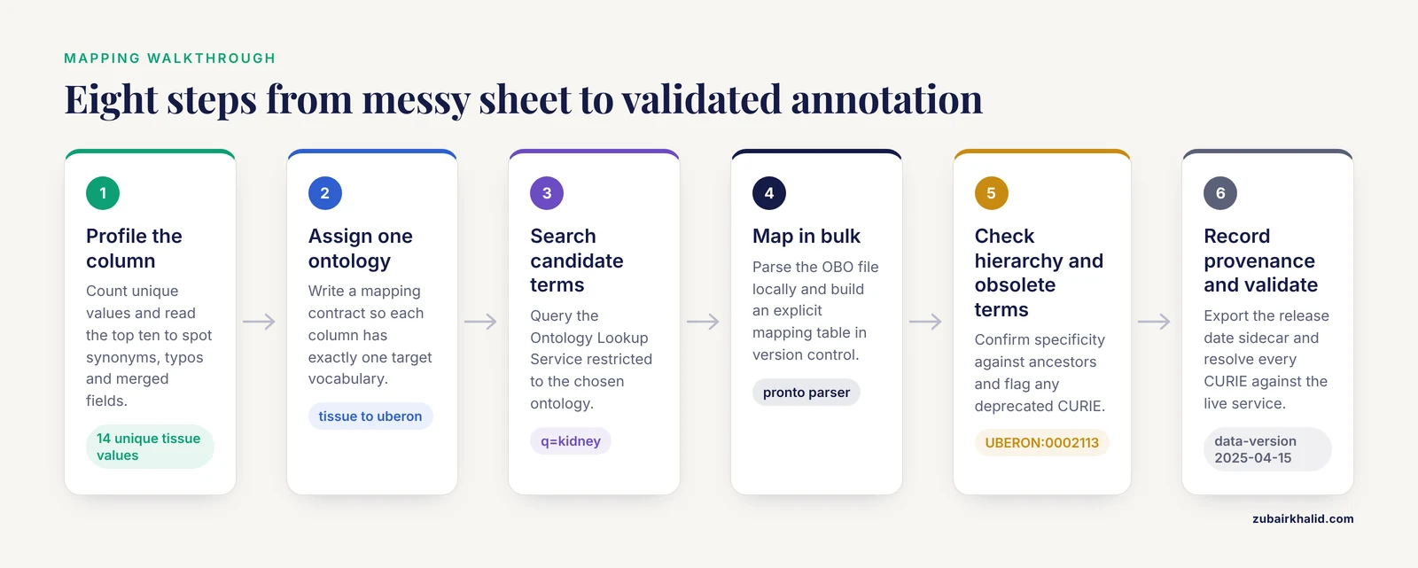
This walkthrough uses a realistic scenario: a lab holding a combined sample sheet from several sequencing studies, with columns SampleID, tissue, diagnosis, collection_site, and assay, all filled in by different people over several years. The goal is a validated, ontology-annotated sheet. Each step gives the command, the expected output, and the parameter that matters.
Step 1. Profile the metadata before you touch an ontology
Never start mapping on sight. Profile the actual values first, because the profile tells you whether you face a synonym problem (many labels, one concept), a typo problem (near-duplicates), or a structural problem (values merged into the wrong column).
import pandas as pd

samples = pd.read_csv("sample_sheet_raw.csv", dtype=str)

for col in ["tissue", "diagnosis", "collection_site"]:
    print(f"== {col} ==")
    print("unique values:", samples[col].nunique(dropna=False))
    print(samples[col].value_counts(dropna=False).head(10))
Expected output for the tissue column of a urology-adjacent cohort:
== tissue ==
unique values: 14
kidney            412
Kidney            187
KIDNEY             96
kidney             41
renal cortex       33
kidney tumor       28
Kidnay             12
renal mass          7
NaN                 6
renal cortex+fat   3
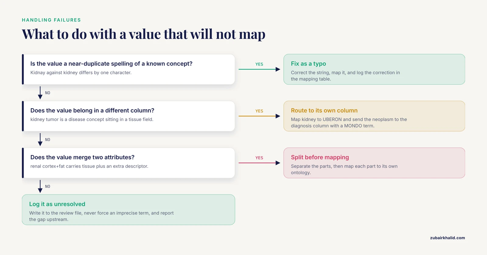
Read that output the way the large-scale curators learned to read it. kidney, Kidney, KIDNEY, and kidney (trailing space) are one concept with four spellings. Kidnay is a typo. kidney tumor and renal mass are misplaced values, disease concepts sitting in a tissue column, and this exact failure class is one of the recurring quality issues documented during curation of 212,027 public samples [1]. renal cortex+fat is merged information across attributes. Each failure class needs a different treatment, and profiling is how you see which ones you have.
Step 2. Assign one target ontology to each column
Write the assignment down as a small dictionary in your pipeline code. This is your mapping contract.
target_ontologies = {
    "tissue":          "uberon",
    "diagnosis":       "mondo",
    "phenotype":       "hp",
    "assay":           "edam",
    "collection_site": "gaz",
}
Do not allow two ontologies for one column within a project. Mixed-vocabulary columns are the single largest source of downstream integration pain, because every consumer then needs a crosswalk between vocabularies that may not exist.
Step 3. Find candidate terms with the Ontology Lookup Service
The EBI Ontology Lookup Service (OLS) exposes a search API over most OBO ontologies. Use it interactively while you build the mapping dictionary. The query runs over labels and synonyms.
curl "https://www.ebi.ac.uk/ols4/api/search?q=kidney&ontology=uberon&fieldList=iri,label,obo_id"Expected output (trimmed to the relevant fields):
{
  "response": {
    "docs": [
      {
        "iri": "http://purl.obolibrary.org/obo/UBERON_0002113",
        "label": "kidney",
        "obo_id": "UBERON:0002113"
      },
      {
        "iri": "http://purl.obolibrary.org/obo/UBERON_0000362",
        "label": "renal cortex",
        "obo_id": "UBERON:0000362"
      }
    ]
  }
}
The parameter that matters here is ontology, which restricts the search so you do not get a "kidney" cell type from a different vocabulary mixed into your candidates. When two candidates differ in specificity, such as kidney versus renal cortex, prefer the term that matches what was actually sampled, and record the decision.
Step 4. Load the ontology locally and map in bulk
For repeatable bulk mapping, download the ontology file once and parse it with pronto, a pure-Python OBO and OWL parser.
from pronto import Ontology

uberon = Ontology("http://purl.obolibrary.org/obo/uberon.obo")

matches = {}
for term in uberon.terms.values():
    if "kidney" in term.name.lower():
        matches[term.id] = term.name

for tid, name in sorted(matches.items())[:8]:
    print(tid, name)
The download is large, on the order of tens of megabytes, and parsing takes a minute on a laptop. Expected output:
UBERON:0000362 renal cortex
UBERON:0002113 kidney
UBERON:0004538 kidney calyx
...
With candidate terms confirmed, build the explicit mapping table. The key discipline is that the mapping lives in a version-controlled file, not in someone's head.
import pandas as pd

raw_values = ["kidney", "Kidney", "KIDNEY", "kidney ", "renal cortex",
              "kidney tumor", "Kidnay", "renal mass", "renal cortex+fat"]

# Concepts resolvable now, one row per distinct concept
mapping = {
    "kidney":        "UBERON:0002113",
    "renal cortex":  "UBERON:0000362",
    "renal mass":    "UNRESOLVED_DISEASE_IN_TISSUE_COLUMN",
    "kidney tumor":  "UNRESOLVED_DISEASE_IN_TISSUE_COLUMN",
    "Kidnay":        "UNRESOLVED_TYPO",
    "renal cortex+fat": "SPLIT_REQUIRED",
}

norm = samples["tissue"].str.strip().str.lower()
samples["tissue_curie"] = norm.map(mapping)

unresolved = samples[samples["tissue_curie"].str.startswith(("UNRESOLVED", "SPLIT"), na=False)]
unresolved.to_csv("unresolved_tissue_values.csv", index=False)
Two design decisions are embedded here and both matter.
First, unresolvable values go to a review file rather than being force-mapped to a nearby term. When the HPO evaluation in the autoimmune cohort found five patient features with no existing term, the correct response was to report the gap, not to shoehorn the features into imprecise terms, because imprecise terms then corrupt gene prioritization downstream [2]. Your unresolved file is the raw material for exactly that kind of feedback to ontology maintainers, and the HPO refinement work in SARDs shows such feedback producing concrete term corrections [2].
Second, the mapped column keeps CURIEs (compact URIs such as UBERON:0002113) and the original free-text column stays in the sheet. Every serious harmonization effort keeps raw values alongside harmonized ones, because a better ontology release next year should let you re-map without recovering the original data [1].
Step 5. Check the hierarchy so you do not annotate too narrowly
An ontology is not a flat list. Before finalizing a term, look at its ancestors and descendants to confirm the specificity is right for your question.
term = uberon["UBERON:0002113"]
print(term.name)
for parent in term.superclasses(distance=2):
    print(" parent:", parent.id, parent.name)
Expected output:
kidney
 parent: UBERON:0000362 renal cortex...
 parent: UBERON:0000064 organoblast...
 parent: UBERON:0004120 mesenchymal tissue...
 parent: UBERON:0005177 adnexal organ...
...
If your study genuinely sampled whole kidney, UBERON:0002113 is correct. If the biopsies were cortical biopsies, annotating UBERON:0000362 preserves information that a downstream query for cortex would otherwise lose. Annotating at the right level of specificity is one of the highest-value tips in genomics ontology sample annotation, because specificity lost at annotation time cannot be recovered by analysis.
Step 6. Check for deprecated terms
Terms get obsoleted and replaced. pronto exposes the flag directly.
def check_obsolete(curie):
    t = uberon[curie]
    if t.obsolete:
        repl = t.replaced_by or "no replacement recorded"
        print(f"DEPRECATED {curie} -> {repl}")
    else:
        print(f"OK {curie} ({t.name})")

check_obsolete("UBERON:0002113")
Expected output:
OK UBERON:0002113 (kidney)Run this check over every mapped CURIE in the sheet as part of continuous integration, not just once. Ontology releases regularly obsolete terms, and an annotation set built against a release from three years ago can silently contain dead identifiers.
Step 7. Record provenance and export
Export both the CURIE column and a small sidecar recording the ontology versions used.
versions = {
    "uberon": uberon.metadata["data-version"],
    "annotation_date": "2026-11-11",
    "mapping_table": "mappings_tissue_v3.csv",
}
import json
with open("annotation_provenance.json", "w") as fh:
    json.dump(versions, fh, indent=2)

samples.to_csv("sample_sheet_annotated.csv", index=False)
Expected annotation_provenance.json:
{
  "uberon": "2025-04-15",
  "annotation_date": "2026-11-11",
  "mapping_table": "mappings_tissue_v3.csv"
}
The data-version field is the release date stamped inside the OBO file header. That single string is what makes the annotation reproducible.
Step 8. Validate the whole sheet programmatically
A validation script that resolves every CURIE against the live OLS catches dead identifiers, prefix typos, and terms that were mapped but never loaded.
import requests
from urllib.parse import quote

def validate(curie):
    url = ("https://www.ebi.ac.uk/ols4/api/search?q="
           + quote(curie) + "&queryFields=obo_id&fieldList=obo_id,label")
    hits = requests.get(url, timeout=30).json()["response"]["docs"]
    return any(h.get("obo_id") == curie for h in hits)

for curie in samples["tissue_curie"].dropna().unique():
    if curie.startswith("UBERON"):
        print(curie, "VALID" if validate(curie) else "NOT FOUND")
Expected output:
UBERON:0002113 VALID
UBERON:0000362 VALID
This is also your safety net against the most common silent failure in hand-built mapping tables: the term that looks plausible, is never checked, and does not exist.
Sample Identifiers That Carry Semantics
Controlled terms in a metadata table are one layer. The identifiers themselves are another. Most labs track subjects and biospecimens with simple IDs or UUIDs, which guarantee uniqueness but embed no semantic information, forcing integration, cohort selection, and analysis to go back to a separate metadata table every time. ClarID is a recent, open, domain-agnostic specification designed to close that gap with two formats: a human-readable form such as CNAG_Test-HomSap-00001-LIV-TUM-RNA-C22.0-TRT-P1W, encoding project, species, subject, tissue, disease status, assay, and timepoint, and a compact "stub" form such as CT01001LTR0N401T1W, optimized for filenames, pipeline logs, and physical labels. ClarID-Tools, the reference implementation, processes tabular metadata in CSV or TSV, uses a YAML codebook to generate, decode, and validate identifiers, and supports bulk and single-sample processing as well as QR code creation and reading [3].
The YAML codebook is where ontologies meet identifiers. You define controlled vocabularies per field, and the tool enforces them:
species:
  HomSap: human
tissue:
  LIV: liver
  KID: kidney
assay:
  RNA: RNA-seq
disease:
  TUM: tumor
  NRM: normal
This approach has a specific advantage over hard-coding identifiers in scripts: the codebook is a data file, versioned alongside your metadata, and decoding an identifier back into its fields is a deterministic operation. For teams managing genomics data storage across archives and working directories, human-readable identifiers dramatically reduce the sample mix-ups and join errors that pure UUID workflows invite.
Functional Annotation: Choosing the Right Tool for the Genome
Once sample metadata is under control, the gene-level layer needs annotation too, and here tool choice is an evidence question rather than a preference. The first large-scale benchmark of four prominent open-source prokaryotic annotation tools, Prokka, Bakta, EggNOG-mapper, and PGAP, ran across 156,033 diverse genomes, including Escherichia coli strains for baseline performance, thousands of archaeal and bacterial genomes, and frameshifted and metagenome-assembled genomes. The findings map cleanly onto genome quality: Bakta performed best on high-quality bacterial genomes, while PGAP was better for archaeal genomes and for challenging bacterial assemblies including metagenome-assembled, fragmented, or contaminated samples. For Gene Ontology annotation specifically, PGAP consistently provided broader term coverage, whereas EggNOG-mapper offered more terms per feature [4].
| Tool | Best suited to | GO term behavior |
|---|---|---|
| Bakta | High-quality bacterial genomes | Standard output |
| PGAP | Archaeal genomes, MAGs, fragmented or contaminated assemblies | Broader GO term coverage |
| EggNOG-mapper | Feature-rich functional summaries | More terms per feature |
| Prokka | Fast draft annotation | Standard output |
The benchmark's own framing is the right one for your pipeline decisions: select the tool based on genome quality, taxonomy, and origin, including whether the assembly is a metagenome-assembled genome (MAG) [4]. A pipeline that annotates contaminated assemblies with a tool benchmarked only on clean isolates is producing GO terms whose accuracy nobody has measured.
Downstream Enrichment: Where the Annotation Pays Off
Sample-level and gene-level annotation converge in functional enrichment analysis. The GO terms attached to your gene set are only as good as the annotation layer beneath them, and for well-annotated model organisms, mainstream tools such as g:Profiler, DAVID, and GOrilla work well. For non-model organisms, particularly bacteria and other microorganisms, curated functional annotations are often scarce, and the common workaround, transferring annotations from related species by homology with tools like BLAST, introduces annotation errors and misses species-specific functions [5].
A published protocol addresses this directly by walking through building custom annotation R packages from genomic data retrieved from NCBI. The resulting packages import into R as libraries and work directly with clusterProfiler, enabling GO and pathway enrichment on organisms that have no off-the-shelf annotation resource. The demonstration organism was Mycobacterium tuberculosis H37Rv, applied to differentially expressed genes from the rifampicin-response dataset GSE292409 [5].
The core clusterProfiler call against such a custom package looks like this:
library(clusterProfiler)

ego <- enrichGO(
    gene          = deg_list,
    OrgDb         = org.MtbH37Rv.eg.db,
    ont           = "BP",
    pAdjustMethod = "BH"
)

head(as.data.frame(ego))
Expected output is a data frame of enriched Biological Process terms with adjusted p-values, one row per enriched GO term. The parameters that matter are ont, which selects the GO branch, and pAdjustMethod, where Benjamini-Hochberg ("BH") is the standard multiple-testing correction for enrichment contexts.
At the applied end of the spectrum, a systematic review of synovial fluid proteomic biomarkers in knee osteoarthritis shows the whole chain working together. Seven studies met inclusion, reported biomarkers including Cathepsin G (CTSG), angiotensinogen (AGT), periostin (POSTN), haptoglobin (HP), complement components, and matrix proteins such as ADAMTS4 and LYVE-1. Functional annotation with ShinyGO revealed enrichment in glycosaminoglycan binding, complement cascades, and redox pathways, and protein-protein interaction analysis with STRING version 12.0 identified central hub nodes including COL1A1, ACAN, COMP, and POSTN alongside matrix-degrading enzymes MMP1, MMP3, and MMP13, painting a picture of tightly connected extracellular matrix remodeling [6]. The enrichment results were only interpretable because the protein identifiers were resolved to annotation terms first, which is the same discipline, one level up the pipeline, as mapping a tissue string to a UBERON CURIE.
Storage and Infrastructure for Annotated Metadata
Annotation without a storage plan evaporates. Three layers cover most needs in bioinformatics data management.
The first layer is the annotation itself: paired columns of raw values, mapped CURIEs, and a provenance sidecar recording ontology versions, as built in the walkthrough. This travels with the data everywhere, survives format migrations, and is the minimum any reviewer or collaborator needs.
The second layer is queryable access across many studies. When you face hundreds of studies rather than one sample sheet, the harmonized resources built by others become infrastructure. The OmicsMLRepoR Bioconductor package exposes the metadata harmonized across curatedMetagenomicData and cBioPortal, 212,027 samples in total, enabling repository-wide queries and cross-study analyses that were previously impractical with heterogeneous metadata [1]. Before building your own harmonization layer, check whether a resource like this already covers your domain, because retrospective curation at that scale is expensive and partly done.
The third layer is structured file formats that keep semantics machine-readable at rest. ISA-Tab and MIxS-style formats capture investigation and sequencing context in a tabular structure with controlled vocabularies, and JSON-LD adds linked-data semantics for pipelines that want to query metadata as a graph. Whatever format you choose, the invariant is the same: identifiers resolve, ontology versions are recorded, and raw values survive alongside mapped terms.
Common Mistakes and Limitations
These are the failures that recur across projects, drawn from documented large-scale experience and the source literature.
- Mapping disease values into tissue columns. Values like
kidney tumorin a tissue field are misplaced values, one of the recurring quality issues found across 212,027 public samples [1]. The fix is column-level logic: mapkidneyto UBERON and route the neoplasm concept to the diagnosis column, which gets its own MONDO term. Forcing a single term to carry two concepts destroys both.
- Trusting label similarity over meaning.
Kidnayandkidneydiffer by one character but only one is a concept. Profiling, typo triage, and explicit human sign-off on the mapping table are what large harmonization efforts relied on, and automation alone did not resolve their conflicting annotations [1]. Treat string similarity as a suggestion engine, never as the mapper itself.
- Assuming the ontology has a term for everything. In the SARD cohort evaluation, 36.9 percent of patients had at least one missing HPO term and five features could not be mapped at all [2]. Every pipeline needs an unresolved-values queue, and someone responsible for reporting those gaps upstream.
- Over-annotating through homology. Transferring GO terms from a related species by BLAST is the default for non-model organisms and it injects errors while missing species-specific biology [5]. A custom annotation package built from NCBI data for the organism of interest is the sturdier path.
- Annotating MAGs and messy assemblies with tools benchmarked on clean isolates. PGAP outperformed on archaeal genomes and on metagenome-assembled, fragmented, or contaminated bacterial assemblies, while Bakta led on high-quality bacterial genomes. Matching tool to genome quality is now an evidence-based decision, not a habit [4].
- Writing ontology IDs without raw values. If you store only
UBERON:0002113and discardkidney tumor, you cannot re-map when the ontology improves or when you realize the original annotation conflated two concepts. Keep both, always.
- Ignoring version drift. Ontologies change. An annotation set without a recorded release date is irreproducible by construction, and terms can be deprecated between releases, as the obsolete-term check in Step 6 exists to catch.
- Hard-coding semantics into free-text identifiers. Ad hoc identifiers like
sample1_KIDNEY_tumor_final_v2encode semantics inconsistently and break parsers. A specification like ClarID, driven by a versioned YAML codebook and validated by its tooling, gives you the same human readability with machine-checkable structure [3].
One honest limitation of the whole approach: ontology mapping does not create information that was never recorded. If collection site was never written down, no ontology recovers it. Annotation improves findability, comparability, and reusability of what exists. Gaps in collection practice remain gaps.
Frequently Asked Questions
What is an ontology in genomics metadata?
An ontology is a structured vocabulary in which biological and biomedical concepts receive stable identifiers and explicit relationships, such as UBERON for anatomy, HPO for phenotypes, and GO for gene functions. In metadata, it replaces free-text labels like "kidney" or "tumor" with resolvable CURIEs such as UBERON:0002113, so that filtering, joining, and cross-study comparison become reliable string-free operations.
Which ontologies should I use for sample annotation?
Match one ontology to each column: UBERON for tissue, MONDO or Disease Ontology for diagnosis, HPO for human phenotypes, GO for gene function, and EDAM or MIxS for assay and sequencing context. Keep the assignment in a version-controlled mapping contract, and do not mix two vocabularies for the same column within a project.
How do I map free-text metadata to ontology terms step by step?
Profile the column to classify its problems, assign a target ontology, search candidate terms through the Ontology Lookup Service, load the ontology locally with a parser such as pronto, build an explicit mapping table in version control, check term specificity against the ontology hierarchy, flag obsolete terms, record the ontology release date in a provenance file, and validate every CURIE programmatically. Values that cannot map go to a review file, never to a guessed term.
Do I need to annotate genes with GO terms myself?
Usually no, because annotation tools do it for you, but the tool matters. A benchmark across 156,033 prokaryotic genomes found PGAP gave broader GO term coverage while EggNOG-mapper gave more terms per feature, with Bakta strongest on high-quality bacterial genomes and PGAP better for archaeal and messy assemblies such as MAGs. Pick the tool by genome quality and taxonomy, not by habit.
What do I do when no ontology term exists for my value?
Log it in an unresolved-values file rather than forcing an imprecise mapping. Missing terms are a documented reality, with 36.9 percent of patients in one autoimmune disease cohort lacking at least one HPO term and five features having no term at all, and imprecise mappings demonstrably distort downstream tools such as gene variant prioritization. Report the gap to the ontology maintainers, since community feedback produces term additions and corrections.
How do I handle metadata from public repositories?
Expect heterogeneity and plan for retrospective harmonization, because most published omics data remains in non-standardized formats. Before curating from scratch, check existing resources such as the OmicsMLRepoR package, which provides harmonized metadata for 212,027 samples across curatedMetagenomicData and cBioPortal and supports repository-wide queries that heterogeneous raw metadata makes nearly impossible.
Should I encode metadata in my sample identifiers?
You can, if you do it with a specification rather than ad hoc strings. ClarID defines both a human-readable format encoding fields like species, tissue, disease, and assay, and a compact stub format for filenames and labels, with an open-source tool that generates, decodes, and validates identifiers from a YAML codebook applied to CSV or TSV metadata. UUIDs guarantee uniqueness but carry no semantics, which pushes every integration task back to a metadata lookup.
How do I keep annotations valid as ontologies evolve?
Record the ontology release date with every annotation batch, re-run obsolete-term checks on each new release, keep raw values alongside CURIEs so you can re-map, and treat the mapping table as a versioned artifact with named revisions. When a release obsoletes a term you use, the check will surface its recorded replacement, and you re-run the mapping rather than patching identifiers by hand.
Sources
- Large-scale manual curation and harmonization of metadata from metagenomic and cancer genomic repositories: challenges and solutions.
- Refining Human Phenotype Ontology (HPO) to enable better phenotype-genotype integration in systemic autoimmune rheumatic diseases.
- ClarID: a human-readable and compact identifier specification for biomedical metadata integration.
- Large-scale benchmarking of prokaryotic annotation tools across thousands of species.
- Enhanced RNA-Seq Expression Profiling and Functional Enrichment in Non-model Organisms Using Custom Annotations.
- Synovial Fluid Proteomic Biomarkers in Knee Osteoarthritis: A Systematic Review and Gene Ontology Analysis.