Genomics Data Storage Requirements: How to Calculate Them
By Dr. Zubair Khalid, DVM, MS, PhD ·
By the end of this article you will be able to estimate, with defensible numbers, how much disk capacity a genomics project needs across scratch, primary, backup, and archive tiers, and you will be able to verify that estimate against files that already exist on your system. You will need access to a Linux or macOS shell, the samtools package installed for alignment file work, and either the real FASTQ files from a pilot run or a directory of similar historical data you can measure. Everything else is arithmetic you can do in a spreadsheet.
Underestimating genomics data storage is one of the most common and most expensive planning failures in bioinformatics. Sequencing output keeps growing, and that growth forces laboratories to build robust infrastructure for storage, processing, and interpretation of very large datasets [1]. National-scale genomics programs now treat data management as an explicit line item when they cost sequencing and bioinformatics capacity, which means storage estimates end up in budgets and grant applications, not just in the head of the person running the cluster [2]. A structured estimate protects you from the two failure modes that matter: running out of space mid-pipeline, and buying capacity you never use.
Why Storage Estimates Fail
Most failed estimates share the same root causes. The planner counts only the final deliverable, such as a variant call file, and forgets the intermediate files that are three to ten times larger. The planner counts only one copy of the data and forgets that backup, archive, and working copies all consume the same physical disks. The planner confuses decimal and binary units, or forgets that filesystems, metadata, and RAID layouts eat a meaningful fraction of nominal capacity. Finally, the planner treats storage as a single number when it is really four numbers: scratch space, primary space, backup space, and archive space, each with its own growth rate and retention policy.
The stakes scale with the science. Genomic newborn screening programs, for example, explicitly identify data storage volume and privacy as one of the key implementation themes they must resolve before scaling up [3]. Institutions building high-performance computing capacity in resource-limited settings report that optimized storage and networking configurations are what make high-throughput genomic workflows feasible at all, and they treat storage planning as a deliberate design activity with documented operational rules rather than an afterthought [4]. The rest of this article gives you the same kind of structure: a formula, per-file size models, a worked example, and the commands to verify everything against reality.
Units and Counting Conventions
Before any arithmetic, fix your units. Genomics mixes two counting systems and vendors exploit the confusion.
A base pair of DNA sequence is stored in a FASTQ file as one byte of sequence plus one byte of base quality, with a small per-read header. File sizes on disk are reported in bytes. Storage vendors sell capacity in decimal gigabytes and terabytes, where 1 TB equals 10^12 bytes. Operating systems report usage in binary units, where 1 TiB equals 2^40 bytes, roughly 1.099 TB. The difference is about 10 percent per step. A disk sold as 100 TB shows about 90.9 TiB before any filesystem overhead, and less after formatting. Always do your arithmetic in bytes or decimal GB and TB, then convert once, at the end, to the vendor units you will actually purchase. State which convention you used in your estimate document, because a 10 percent discrepancy between two spreadsheets is a classic source ofArguments during procurement.
Filesystem overhead is real. Filesystem metadata, journaling, reserved blocks, and RAID or erasure-coding parity all consume capacity that df will not show as available for your data. A practical planning factor is 10 to 20 percent of nominal capacity lost before your first file lands, and you should verify the actual fraction on your own system with df -h after formatting a volume. Exact parity overhead depends on your RAID level or erasure-coding configuration, so treat it as a measured quantity, not a constant.
Per-File-Type Size Models
The genomics data storage requirements formula works on file types, because each format has a different relationship between bases sequenced and bytes stored. Start from the fundamental relation:
B_total = C × Gwhere C is average sequencing coverage (reads covering each base, counted once) and G is the reference genome size in bases. For a 30x human whole-genome sample with a 3.1 billion base reference:
B_total = 30 × 3,100,000,000 = 93,000,000,000 bases (93 Gbp, combined across both reads of each pair)From there, each file type scales differently.
FASTQ
An uncompressed FASTQ record contains a header line, the sequence, a separator line, and the quality string. Per base, uncompressed FASTQ costs roughly 2 bytes plus header overhead. Gzip compression typically brings the on-disk cost to between 0.3 and 0.6 bytes per base, depending on sequencing platform, quality-string complexity, and adapter content. The model is:
FASTQ_bytes ≈ B_total × b_pbwhere b_pb is your measured bytes-per-base factor. Never assume a published value. Measure it once on your own instrument and pipeline (shown below), because the factor varies more between platforms than most people expect. For the 93 Gbp example, a measured b_pb of 0.58 predicts about 54 GB of compressed FASTQ per sample. That is in line with the rough practical range for 30x human whole-genome data.
SAM, BAM, and CRAM
SAM is the plain-text alignment format, BAM is its compressed binary form, and CRAM is a more aggressive format that stores alignments relative to a reference sequence. A useful model for BAM is per-alignment-record cost:
BAM_bytes ≈ N_reads × s_record
N_reads = B_total ÷ read_length
For a 150 bp read, 93 Gbp gives about 620 million read pairs, or 1.24 billion alignment records. Compressed BAM records typically cost on the order of 60 to 100 bytes each once you include quality strings, tags, and the per-record index structure, which puts a 30x human BAM near 100 GB. CRAM, when written against the same reference used for alignment, commonly lands near half the BAM size or better. Convert your own numbers rather than trusting any fixed ratio, and always store the reference checksum alongside CRAM files, because CRAM is only decodable with a compatible reference.
VCF, BCF, gVCF, and array formats
Variant call files scale with the number of variants and, for joint calls, with the number of samples, so cohort size dominates. Compression and format choice matter enormously here. In a published benchmark on 1000 Genomes Phase 3 data, the same variant content stored as VCF occupied 14.0 GB, as binary BCF 12.3 GB, and as the array-oriented SeqArray (GDS) format 2.6 GB, meaning the specialized array format was more than five times smaller than plain VCF while also supporting faster parallel access to genotypes [5]. Per-sample gVCF files, which include reference blocks at every position, are individually large relative to their information content, commonly on the order of a few gigabytes per genome compressed, so cohort joint-calling workflows should plan to retain gVCFs only as long as needed and then consolidate.
The general lesson from the variant-call literature extends beyond genotypes. Restructuring genotype and phenotype data to remove redundancy has been shown to cut disk requirements by 86 percent while also speeding analysis dramatically, in one published comparison by a factor of over 6,000 [6]. Format choice is a storage decision, not just a software preference.
Specialized long-read and epigenetic formats
Long-read methylation workflows produce some of the largest per-sample datasets in current genomics, and purpose-built formats exist to control that growth. The CH3 format, designed for modified-nucleotide calls, reduces file sizes by more than 95 percent compared with standard storage of the same data, according to its description alongside the ModSeqR package [7]. If your pipeline emits modified-base calls, check whether an equivalent compressed format exists before you budget for raw output.
Summary table of size models
| File type | Stores | Scaling model | Typical magnitude for one 30x human WGS sample |
|---|---|---|---|
| FASTQ (gzip) | Raw reads and qualities | B_total × b_pb, measure b_pb yourself | ~40 to 70 GB |
| SAM | Alignments as text | ~10x BAM, never retain | hundreds of GB to TB |
| BAM | Compressed alignments | N_reads × s_record, s_record ≈ 60 to 100 bytes | ~80 to 120 GB |
| CRAM | Alignments vs reference | commonly about half of BAM or less | ~40 to 60 GB |
| gVCF | Per-sample genotypes plus reference blocks | scales with genome positions | low single-digit GB |
| Joint VCF (cohort) | Variant matrix | scales with variants × samples | 14.0 GB for 1000 Genomes Phase 3 [5] |
| BCF | Binary VCF | slightly smaller than VCF | 12.3 GB for the same cohort [5] |
| SeqArray GDS | Array-oriented genotypes | highly compressed, parallel access | 2.6 GB for the same cohort [5] |
The exact values in your environment will differ. The purpose of the table is to give you a sanity envelope, and the commands later in this article show you how to replace every typical value with a measurement.
The Genomics Data Storage Requirements Formula
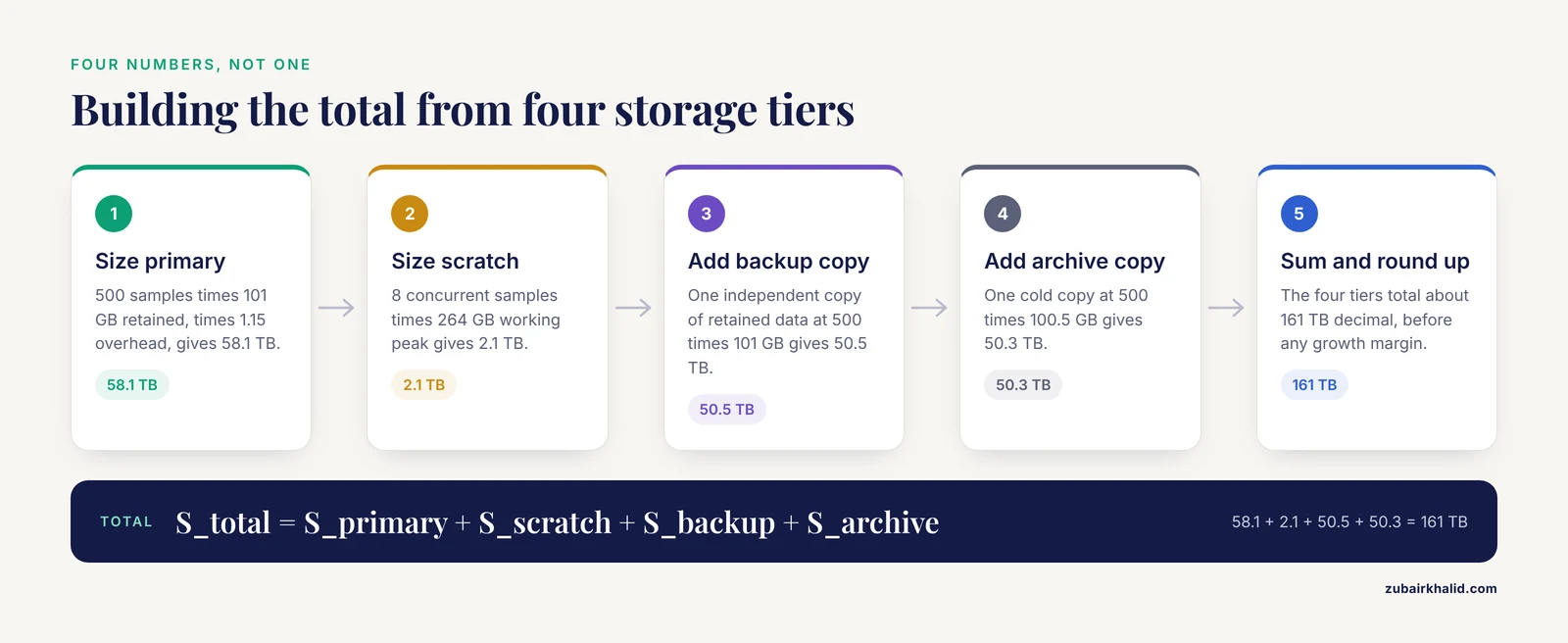
The full genomics data storage requirements formula has four additive terms, each matching a storage tier:
S_total = S_primary + S_scratch + S_backup + S_archive

S_primary = N × s_retained × (1 + f_overhead)
S_scratch = C_concurrent × s_working_peak
S_backup  = C_backup × N × s_retained_backup
S_archive = C_archive × N × s_archive
Define every variable explicitly before you plug in numbers:
Nis the number of samples retained per planning period, usually per year.s_retainedis the per-sample retained footprint in primary storage, the sum of every file type you keep after the pipeline completes.f_overheadis the filesystem and RAID overhead fraction you measured on your own system, commonly 0.10 to 0.20.C_concurrentis the number of samples processed simultaneously at peak, which is set by your scheduler, not your ambitions.s_working_peakis the largest combined footprint of all intermediate files for one in-flight sample, typically FASTQ plus unsorted BAM plus sorted BAM before CRAM conversion.C_backupandC_archiveare the number of independent copies you keep in backup and archive tiers. A defensible default is one backup copy and one archive copy of raw and final data.s_retained_backupands_archivecan be smaller thans_retainedif you exclude intermediates and reports from those copies.
If you prefer a single-line version for a spreadsheet, the compressed form is:
S_total = N × s_retained × (1 + f_overhead + C_backup + C_archive) + C_concurrent × s_working_peakNote what the formula deliberately excludes. It does not include transient files already counted inside s_working_peak, and it does not include compressed-on-the-fly formats. It also does not include the metadata databases, sample sheets, and audit logs that bioinformatics data management requires, which are usually negligible in bytes but not in planning effort.
Genomics Data Storage Requirements Worked Example
This worked example plans for a laboratory that sequences 500 human whole-genome samples per year at 30x coverage, processing up to 8 samples concurrently. Follow the five steps in order. Every command is real and every expected output is realistic for this scenario, but replace the numbers with your own measurements.
Step 1. Measure the bytes-per-base factor on real data
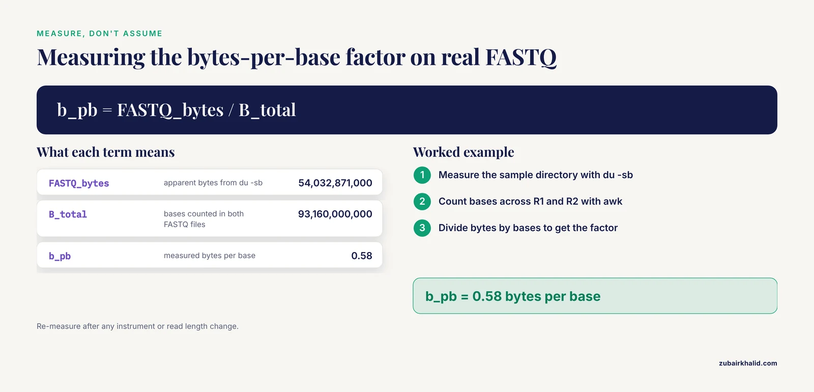
Take one completed sample directory and measure it exactly in bytes:
du -sb /data/raw/sample_A
# 54032871000  /data/raw/sample_A
du -sb reports apparent bytes, which is what you want for capacity math (the plain du -sh reports block-allocated size, useful for a quick sanity check but noisier). Now count the actual bases in the paired FASTQ files:
zcat /data/raw/sample_A/sample_A_R1.fastq.gz /data/raw/sample_A/sample_A_R2.fastq.gz \
  | awk 'NR%4==2 { total += length($0) } END { print total }'
# 93160000000
Compute the factor:
awk 'BEGIN { print 54032871000 / 93160000000 }'
# 0.58
So this instrument and pipeline produce compressed FASTQ at 0.58 bytes per base. Write that number into your planning spreadsheet. It is the single most valuable measurement in the whole exercise, and it takes ten minutes to obtain.
Step 2. Model the retained per-sample footprint
Using B_total = 93 Gbp and the measured factor:
FASTQ (gzip)      = 93e9 × 0.58        ≈ 54 GB
CRAM (vs GRCh38)  ≈ 45 GB               (converted and measured, see Step 4)
gVCF (compressed) ≈ 1.5 GB
QC reports, logs  ≈ 0.1 GB
s_retained        ≈ 100.6 GB ≈ 101 GB per sample
If your pipeline still retains sorted BAM instead of CRAM, replace the 45 GB with roughly 100 GB and watch the total double. This is the single highest-leverage format decision in the plan.
Step 3. Model the working peak for one concurrent sample
Walk through your pipeline and list what exists on disk simultaneously at the worst moment, usually just after sorting the BAM and before CRAM conversion and scratch deletion:
FASTQ input              54 GB
Unsorted BAM            100 GB
Sorted BAM              100 GB
Sort temporaries         10 GB (approximate, depends on sorter memory settings)
s_working_peak ≈ 264 GB
If you pipe your sorter output directly into CRAM conversion without materializing the sorted BAM, s_working_peak drops by 100 GB per concurrent slot, which at 8 slots is nearly a terabyte of scratch you never need to buy. Pipeline design and storage design are the same conversation.
Step 4. Convert and verify the CRAM size
The CRAM estimate should be measured, not assumed:
samtools view -C -T GRCh38.fa -o sample_A.cram sample_A.sorted.bam
du -sb sample_A.cram
# 44800000000  sample_A.cram
samtools quickcheck sample_A.cram && echo OK
# OK
quickcheck validates the BGZF structure and EOF marker, which is the fastest guard against a CRAM silently truncated by a full disk. Record the measured CRAM size per sample and compare it across your first ten samples. If the ratio of CRAM to BAM varies wildly between samples, something is wrong, usually a missing or mismatched reference.
Step 5. Assemble the four tiers and convert to procurement units
S_primary = 500 × 101 GB × 1.15           = 58.1 TB
S_scratch = 8 × 264 GB                     = 2.1 TB
S_backup  = 1 × 500 × 101 GB               = 50.5 TB
S_archive = 1 × 500 × 100.5 GB             = 50.3 TB

S_total  ≈ 161 TB (decimal)
Round up with a growth margin. Persistent primary storage grows by about 50.5 TB per year at this sample volume, so a three-year plan needs roughly 151.5 TB of cumulative primary capacity before overhead and backup growth, and your procurement conversation should be framed in those cumulative terms rather than a single-year snapshot. If your funder asks why the estimate is larger than the size of the deliverable VCF files, the answer is the formula itself: retained raw data plus one backup copy plus one archive copy dominate the total, and they exist so that reanalysis never requires resequencing.
Step 6. Validate against reality
After your pilot batch of 20 samples, compare predicted against measured:
du -sh /data/processed
# 1.98T  /data/processed
Predicted for 20 samples at 101 GB is 2.02 TB, measured 1.98 TB, a 2 percent gap, which is excellent. Gaps larger than about 10 percent mean one of your per-file models is wrong, and you should find out which file type drifted before scaling the estimate to the full run. Keep monitoring weekly during the first months:
df -h /data /scratch
# Filesystem      Size  Used Avail Use% Mounted on
# /dev/md0        120T   55T   62T  47%  /data
# /dev/md1        4.0T  1.9T  1.9T  51%  /scratch
Tracking Use% against your sample-completion schedule turns the estimate into an early-warning system. When actual growth diverges from the plan, the cause is almost always one of the mistakes listed later in this article.
Reducing the Footprint Through Format Choices
Once the estimate exists, the fastest way to shrink it is to change what you store, not how many disks you buy. Three published results anchor this point.
First, variant data belongs in specialized formats. For the 1000 Genomes Phase 3 cohort, converting the same variant calls from VCF to the SeqArray GDS format cut the footprint from 14.0 GB to 2.6 GB while also making genotype retrieval two to three times faster than reading BCF through the htslib C library, and allele-frequency calculation over 16 times faster than vcftools on the VCF [5]. The conversion itself is a single call:
library(SeqArray)
seqVCF2GDS("cohort.vcf.gz", "cohort.gds", verbose = TRUE)
Second, redundant data structures are a hidden tax. The multi-table, normalized data structure described in the genomic data-flood study eliminated redundant copies of genotype and phenotype records and cut required disk space by 86 percent, while making analytical calculations dramatically faster, in that study by a factor of 6,248 [6]. The practical translation for a working laboratory is to normalize any repeated per-sample metadata out of your analysis tables and keep it once in a relational or tabular store.
Third, specialized domains have their own compressed formats. The CH3 format for modified-nucleotide methylation data reduces file sizes by more than 95 percent, and it exists precisely because raw long-read methylation outputs overwhelm ordinary storage budgets [7]. When a well-maintained domain format exists, adopting it is usually cheaper than expanding the array.
The same logic applies at the archive scale. Groups that mine public repositories report that searching within the Sequence Read Archive requires significant time, data storage, and computing power, which is a reminder that archived data you may want to reanalyze has a real retrieval and staging cost, and that keeping your own well-organized compressed archive is often cheaper than repeatedly staging public data at full scale [8].
Storage Tiers, Retention, and Policy
A capacity number is only useful once it is attached to a retention policy. Structure your genomics data storage into four tiers with different media, different growth rates, and different deletion rules.
Scratch tier. High-performance storage sized by C_concurrent × s_working_peak. Scratch is expendable by definition, and pipelines must delete intermediates on completion. In resource-limited settings, the UVRI high-performance computing framework specifically highlights optimized storage and networking configurations as what allows high-throughput genomic workflows to run on constrained infrastructure, and treats disciplined operational rules as the mechanism that keeps the system sustainable [4]. The most important of those disciplines for scratch space is that nothing lives there permanently.
Primary tier. Holds s_retained for every active sample. This is where format choices pay off, because CRAM instead of BAM and GDS instead of VCF shrink this tier directly.
Backup tier. One or more independent copies of raw and final files. Backup exists to survive a primary-tier failure, so it must be on separate hardware, ideally in a separate room or site. It does not need to be fast. It needs to be complete and regularly verified with checksums.
Archive tier. Cold copies of data retained past the active-analysis period, governed by your institutional data-retention policy and any applicable privacy requirements. Genomic screening programs identify data storage and privacy as intertwined policy challenges, because retained genomic data is identifiable data, and retention decisions are therefore governance decisions as much as technical ones [3]. Write the retention schedule down, including which file types are retained, for how long, and who authorizes deletion, before the archive tier fills up.
Governance and Bioinformatics Data Management
Capacity arithmetic is only half of bioinformatics data management. The other half is the system that decides what gets stored, where, in what format, and for how long. Long-running genome databases solved this decades ago with dynamic, scripted database layouts rather than static file dumps. The CBS Genome Atlas database, built on GNU Make, Perl, and MySQL, was designed so that new analyses and changing methods could be added without restructuring the storage, which is exactly the property you want when analysis methods change faster than storage does [9]. The transferable principle is that derived results should be regenerable from scripted pipelines against retained primary data, so that your archive never has to store every intermediate version of every analysis.
Two further governance points come from recent practice. First, capacity planning is now part of formal costing. A multi-country survey conducted to inform the genomics costing tool 2.0 captured data management alongside instrumentation and reagents, because funders expect storage to appear in national genomics budgets with the same rigor as consumables [2]. If your estimate has to survive that kind of scrutiny, keep the formula, the measured parameters, and the validation records in a version-controlled document. Second, storage formats multiply across an institution. A survey of genetic-test result handling across multiple research centers found highly variable storage formats and retrieval methods for genetic results in electronic health records, which made cross-institution analysis slow and error-prone [10]. Inside your own laboratory, the equivalent failure is five folders with five naming schemes and three compression states. A written data-management plan that fixes file naming, directory layout, compression formats, and checksum policy prevents it.
Common Mistakes and Limitations
Counting only final deliverables. The variant call file for a genome is tiny. The FASTQ, alignment files, and working copies are the actual storage load. Always budget from s_retained and s_working_peak, never from the deliverable.
Confusing GB and GiB. A disk marketed as 20 TB holds about 18.2 TiB, and your du totals in GiB will look 10 percent smaller than your spreadsheet in GB. Pick decimal bytes for all planning math and convert once.
Assuming compression ratios from someone else's instrument. The bytes-per-base factor depends on platform, quality encoding, and content. Measure it with the awk one-liner above and re-measure when you change instruments or read lengths.
Forgetting the scratch tier. Pipelines die with No space left on device at the sorting step, which is the moment of peak disk usage. Size scratch from concurrent slots, not from average throughput.
Keeping BAM when CRAM suffices. BAM costs roughly twice the CRAM size for aligned data against a reference. Retaining BAMs across thousands of samples is one of the largest avoidable costs in most laboratories.
Retention without deletion. Archive tiers that only ever grow will eventually consume the entire budget. A retention policy with named deletion events is part of the storage plan, not an optional extra, and it interacts with privacy obligations for identifiable genomic data [3].
Ignoring inodes and small files. Millions of tiny QC and log files can exhaust filesystem metadata capacity before byte capacity runs out. Check with df -i and consolidate small outputs into per-sample archives.
No checksums. Silent corruption during transfer or on aging media is discovered far too late without checksums. Generate a checksum for every retained file at creation and verify at backup and archive boundaries.
Treating the estimate as permanent. Coverage targets, read lengths, cohort sizes, and formats all change. Re-run the estimate annually and after any instrument or pipeline change.
A final limitation. Every magnitude in this article describes standard short-read and long-read sequencing workflows at commonly used coverage levels. Single-cell, very high-coverage clinical, and ultra-long-read projects can shift the per-file constants substantially, so the method stands but the numbers must be re-measured for your specific assay.
Frequently Asked Questions
How do I calculate genomics data storage requirements for a new project?
Start from the formula S_total = S_primary + S_scratch + S_backup + S_archive. Estimate per-sample retained size from measured bytes per base for FASTQ plus your alignment and variant file formats, multiply by sample count for primary, size scratch from concurrent slots times working peak, and add one backup and one archive copy. Validate the per-sample number against a real pilot batch before committing to procurement.
How much storage does one 30x human whole-genome sample need?
Roughly 100 GB retained per sample as compressed FASTQ plus CRAM plus gVCF, with a working peak of about 260 GB during processing if intermediate BAMs are materialized. These are planning magnitudes, and the exact values should be replaced with measurements from your own instrument and pipeline.
Should I store BAM or CRAM files?
Store CRAM for long-term retention, because it commonly lands near half the BAM size when written against the reference used for alignment. Keep a BAM only during active processing if a downstream tool requires it, and record the reference checksum with every CRAM.
How much smaller is SeqArray than VCF for variant data?
In the published 1000 Genomes Phase 3 benchmark, the same variant calls occupied 14.0 GB as VCF and 2.6 GB as SeqArray GDS, a greater than fivefold reduction, with additional speed advantages for genotype retrieval and allele-frequency calculation.
Do I need to back up raw FASTQ files if I keep the BAM files?
Yes. BAM and CRAM files are reconstructions that depend on alignment software, parameters, and for CRAM on a specific reference, so retaining the raw FASTQ in backup and archive tiers is the standard safeguard for reproducibility. The FASTQ tier is also what enables reanalysis with future methods.
What is the difference between GB and GiB in storage planning?
A GB is 10^9 bytes and a GiB is 2^40 bytes, about 9.4 percent larger. Vendors sell in decimal GB and TB while operating systems report in binary units, so plan in decimal bytes and convert once to avoid apparent discrepancies between spreadsheets and df output.
How do I handle storage planning when infrastructure funding is limited?
Adopt the tiered model and spend scarce money on format efficiency first, because converting to CRAM, GDS, and domain-compressed formats reduces every tier at once. Institutions operating large-scale genomics in resource-limited settings report that deliberate storage optimization, open-source tooling, and phased capacity building are what make such programs sustainable.
How often should I re-run my storage estimate?
Re-run it at least annually, and immediately after any change in instrument, read length, coverage target, genome size, pipeline, or retention policy. Track df usage weekly against the predicted growth curve so divergence is caught within one billing cycle rather than one procurement cycle.
Sources
- Transformative Applications and Innovations in Next-Generation Sequencing Data Analysis.
- Next-generation sequencing and bioinformatics capacity: findings from a multi-country survey to guide the genomics costing tool 2.0.
- Key Outcomes from a Stakeholder Workshop on Genomic Newborn Screening: Recommended Next Steps for the Integration of Genomics into Public Health Programs.
- A scalable HPC framework for bioinformatics in resource-limited settings: design principles, implementation, and sustainability from the UVRI experience.
- SeqArray-a storage-efficient high-performance data format for WGS variant calls.
- Damming the genomic data flood using a comprehensive analysis and storage data structure.
- ModSeqR: an R package for efficient analysis of modified nucleotide data.
- Meta-analysis of public raw sequence data unveils the distribution and dynamics of emerging aquatic pathogens: using Macrobrachium rosenbergii golda virus as a case study.
- CBS Genome Atlas Database: a dynamic storage for bioinformatic results and sequence data.
- Finding buried genetic test results in the electronic health record is inefficient and variable across institutions.