Genomics Data Growth Planning: How to Plan for Capacity
By Dr. Zubair Khalid, DVM, MS, PhD ·
Genomics data growth planning is the practice of forecasting how much sequencing data your program will generate, processed, and retain over the next several years, then provisioning storage, compute, and staff so that capacity arrives before the data does. The one-sentence difference that separates programs that succeed from programs that drown is this: reactive buying adds disks after the crisis, while forecast-driven planning sizes storage against a sample-volume projection and a written data lifecycle policy. The rule of thumb for choosing between your options is simple. Keep roughly one to two years of actively analyzed data on fast storage near your compute, tier everything older into cheaper capacity or archive storage, and re-forecast every six months against actual sequencing output.
This article walks through the vocabulary you need, a side-by-side comparison of the main genomics data storage options, the pros and cons of each, a worked sizing method with real arithmetic, three concrete scenarios, and the mistakes that most often sink a bioinformatics data management plan.
Why Genomics Data Growth Breaks Default IT Assumptions
General-purpose IT planning assumes that data volumes grow modestly and predictably. Sequencing violates both assumptions. Next-generation sequencing now spans cancer genomics, rare disease diagnostics, infectious disease surveillance, and precision medicine, and each application generates variant-level and read-level data that must be stored, processed, and interpreted on robust computational infrastructure [1]. The scope of what one laboratory produces keeps widening. Single-cell sequencing, long-read platforms, and multi-omics integration have expanded the field's reach into cellular heterogeneity, structural variation, and systems-level analysis, and each of these modalities multiplies the per-sample data footprint compared with a standard short-read experiment [1].
Demand compounds the technology curve. In clinical settings, genomics has moved from a specialty service to routine testing infrastructure. A decade-long survey of genetic counselors in South Africa documented substantial role diversification, with the proportion of counselors primarily in clinical roles falling from 75 percent in 2013 to 45 percent in 2023 as counselors absorbed laboratory, research, and education responsibilities [2]. That kind of professional expansion is a reliable proxy for expanding test volumes, and expanding test volumes translate directly into storage demand.
A third driver is newer still. Artificial intelligence workloads have become a genuine capacity line item. A comprehensive survey of AI agents in healthcare documented exponential growth in the field and organized it around the perception of multi-modal clinical data, including genomics, alongside agent capabilities and a deployment ecosystem spanning clinicians, researchers, and administrators [3]. Systems that integrate omics data with literature knowledge, such as the OASIS platform for plant stress research, demonstrate how AI pipelines consume large heterogeneous datasets and produce additional derived artifacts that someone must ultimately store and version [4]. When you forecast genomics data growth, you are forecasting for three consumers at once: primary analysis, secondary analysis, and increasingly machine learning pipelines.
The Vocabulary You Need Before You Size Anything
Capacity conversations go wrong when participants use the same words for different things. Fix the definitions first.
Raw data is what the instrument produces. For most short-read sequencing, that means FASTQ files, which hold reads and base-quality scores in a compressed text format. A single lane of a modern flow cell can produce tens of gigabytes within hours.
Aligned data is the output of mapping reads to a reference genome, usually stored as BAM (Binary Alignment Map). BAM files index-able, compressed, and roughly the same size as the FASTQ input or larger depending on read density.
CRAM is a more compressed alignment format that stores reads as differences against a reference genome. Converting BAM to CRAM typically cuts alignment storage roughly in half, which matters at terabyte scale.
Variant data includes VCF (Variant Call Format) files and gVCF files, which store called variants and per-position genotype evidence. These are small relative to reads, often measured in megabytes to a few gigabytes per genome, but they are the data you will reanalyze most often, so tier them carefully.
Derived and summary data covers expression matrices, methylation calls, GWAS summary statistics, and machine learning feature tables. A GWAS analysis pipeline, for example, produces summary-level statistics for traits such as backfat thickness or semen quality that get carried into pleiotropy testing, gene network construction, and Mendelian randomization, none of which requires the原始 reads [5]. Storing summary results separately from reads is one of the cheapest capacity wins available.
Tiers describe storage performance classes. Hot storage is fast and sits next to compute. Warm storage holds data you reference occasionally. Cold storage holds data you must keep but rarely touch.
Working set is the subset of data currently under active analysis. This is the number that should drive your fast-storage purchase, not your total holdings.
Replication factor and erasure coding describe protection overhead. Mirrored copies roughly double raw capacity requirements. Erasure coding achieves similar durability with lower overhead, often around 1.5 times the logical volume depending on configuration.
Object storage is flat, scalable storage accessed over network APIs, exemplified by cloud services and on-premises equivalents. It trades per-file performance for near-unlimited scale.
Metadata is the structured description of samples, runs, and analyses. Without it, archived data becomes unreadable in practice, a failure mode discussed later in the mistakes section.
Side-by-Side Comparison of Genomics Data Storage Options
The table below is the core of this guide. It compares the five realistic options for a sequencing program on the criteria that decide actual purchases.
| Criterion | On-premises NAS / server storage | On-premises HPC parallel filesystem | Cloud object storage (hot tier) | Cloud or tape deep archive | Hybrid tiered strategy |
|---|---|---|---|---|---|
| Best for | Small labs, single-investigator groups | Cores and institutes running pipelines daily | Programs with variable sample volume | Long-term retention, compliance holdover | Programs with steady baseline and bursty peaks |
| Scaling model | Add drives or chassis in discrete steps | Add nodes and disk shelves, capacity and bandwidth scale together | Effectively unlimited, pay per stored gigabyte-month | Very cheap per gigabyte, slow retrieval | Scale each tier independently |
| Analysis performance | Adequate for small workloads | Excellent, designed for many simultaneous readers | Moderate, needs staging near compute | Unsuitable for direct analysis | Good, matches tier to workload |
| Growth handling | Manual, lumpy purchases | Planned expansion cycles | Automatic | Automatic | Policy-driven, automated rules |
| Skills required | Basic systems administration | HPC and storage engineering | Cloud engineering, cost management | Cloud engineering or tape robotics | Both cloud and on-premises skills |
| Main risk | Single-box failure, unplanned outgrowth | Capital intensity, staff dependency | Egress and retrieval charges, sprawl | Retrieval delay and cost surprises | Complexity of managing two estates |
| Exit flexibility | High, data is local | High, data is local | Low to moderate, data movement costs | Low | Moderate |
No single row wins on every criterion, which is why the best genomics data growth planning almost always ends up multi-tiered rather than a single-technology decision.
Option 1: On-Premises NAS and HPC Parallel Filesystems
A network-attached storage (NAS) system is a file server that presents shared folders over the network. It is where most genomics programs start because it requires no contracts, no cloud account, and no new skills beyond routine systems administration.
Pros. Full institutional control over hardware and data location, which simplifies compliance conversations. No per-gigabyte recurring charges. Latency to local compute is minimal. Once purchased, marginal storage costs approach media cost.
Cons. Scaling is lumpy. You buy a shelf of drives when you hit 80 percent capacity, and if sequencing volume doubles, that shelf is wrong in a year. Performance collapses when dozens of pipeline jobs hammer a single controller. Most critically, a NAS purchase is a capacity bet, and genomics data growth punishes bad bets with emergency procurement.
A parallel filesystem extends the same idea for compute-heavy workloads. Systems such as Lustre, BeeGFS, and IBM Spectrum Scale stripe files across many servers so that hundreds of simultaneous pipeline jobs can read and write at aggregate speeds a single NAS cannot approach. If your program runs genomics pipelines daily, the parallel filesystem is not optional equipment, it is the working tier.
The UVRI experience in Uganda illustrates what mature on-premises planning looks like under constraint. The institute built a scalable, modular HPC framework for large-scale genomics and multi-omics analysis by integrating open-source HPC management tools, infrastructure automation, and reproducible configuration management, pairing optimized storage and networking configurations with a phased capacity-building strategy [6]. Two of their findings deserve to be written on the wall of every storage planning meeting. First, structured planning and open-source technologies let a resource-limited institution operate genuinely high-throughput workflows. Second, investment in human capacity is not an afterthought to hardware procurement, it is the load-bearing element, because storage without staff who can operate it is an expensive box of spinning rust [6].
Option 2: Cloud Object Storage
Cloud object storage, such as Amazon S3, Google Cloud Storage, or Azure Blob Storage, stores data as objects in flat namespaces accessed over HTTPS APIs. It is the default answer for programs with unpredictable growth because capacity is not a procurement decision.
Pros. Growth is elastic and instant. Durability is engineered into the service, typically through redundant storage across facilities. Lifecycle rules can automatically move objects between tiers based on age. For collaborations, cloud-native sharing sidesteps the file-transfer friction of on-premises estates. Burst compute beside the data eliminates large data movements during analysis peaks.
Cons. The bill scales with access patterns, not just volume. Egress charges for moving data out, request charges for listing and reading, and retrieval charges on archive tiers can exceed storage charges in a poorly designed pipeline. Data sprawl is the quieter danger, where every pilot project spawns a bucket that nobody deletes. Finally, cloud engineering is a real skill set, and programs that assign it to whoever has spare cycles accumulate both security risks and cost surprises.
The privacy dimension deserves explicit treatment. Reviews of NGS applications flag privacy, data sharing, and equitable access as persistent challenges that must be addressed alongside the technical infrastructure, particularly in resource-limited settings [1]. A cloud migration that solves capacity while creating an uncontrolled copy problem for human genomic data has traded one governance failure for a worse one.
Option 3: Deep Archive and Tape
Deep archive tiers, whether cloud-based (Glacier-class services) or physical tape libraries, store data at the lowest cost per gigabyte in exchange for retrieval times measured in hours and retrieval fees.
Pros. Raw sequencing output is the one asset you can never regenerate without resequencing the sample, so a durable, cheap copy of FASTQ files is non-negotiable. Tape libraries, where an institution already owns them, offer media costs that cloud services struggle to match at petabyte scale, plus an air-gapped copy that ransomware cannot reach.
Cons. Retrieval latency makes archives useless as working storage. Archive retrieval pricing punishes careless lifecycle design. Tape requires robotic infrastructure and vendor relationships that many institutions no longer maintain.
Option 4: Hybrid and Multi-Tier Strategies
A hybrid strategy keeps the working set on-premises near the HPC cluster, pushes completed projects to cloud warm storage, and ages immutable raw data into archive, all governed by automated rules rather than manual copy scripts.
Pros. Each tier does what it is good at. Fast parallel storage serves compute, cloud storage absorbs variable growth, and archive holds the permanent record. Costs track actual access patterns. Failures in one tier do not take down the others.
Cons. You are operating two estates, which doubles the skills burden and creates synchronization problems. Every data movement is an opportunity for checksum errors and version confusion. Without written policy, a hybrid estate decays into the worst of both worlds, an on-premises hoard plus a cloud hoard.
Comparing the Options on the Criteria That Decide Real Choices
The table summarizes capabilities. Five criteria actually decide which mix fits your program.
Growth elasticity. If your sample volume is contractual and steady, on-premises expansion planning works. If volume depends on grants, clinical referrals, or outbreak response, cloud elasticity or a hybrid design prevents both overbuilding and rationing analysis.
Bandwidth versus capacity. Pipelines do not just consume gigabytes, they consume input/output operations. Alignment and variant calling against a large cohort need scratch space that reads and writes at hundreds of megabytes to gigabytes per second in aggregate. A terabyte of slow archive storage is worthless to a running workflow. Buy bandwidth for the working set and capacity for everything else.
Compliance and data governance. Human genomic data carries identifier-linked privacy obligations regardless of where it lives. On-premises storage makes access control an institutional problem. Cloud storage makes it a configuration problem. Both are solvable, but both require written access policies, and clinical programs should treat storage location decisions as part of their compliance design, not an IT detail.
Staff capacity. The UVRI framework paper is explicit that sustaining infrastructure depends on human capacity, phased training, service management practices, and collaboration networks as much as on hardware [6]. A cloud strategy with no cloud engineer fails exactly as surely as an HPC strategy with no HPC administrator.
Time to first result. For a new program, the fastest path to productive analysis is often a modest on-premises working tier plus cloud archive, because it avoids both a capital procurement cycle and the learning curve of running pipelines in the cloud.
How to Forecast Capacity: A Worked Method
Genomics data growth planning becomes tractable when you separate the forecast into five multiplicative factors. The per-sample figures below are order-of-magnitude planning estimates in common use across sequencing cores, intended for first-pass sizing. Verify them against your own instrument output and pipeline before committing a budget.
Step 1: Build a per-sample data footprint table
| Assay | Raw FASTQ per sample | Processed holdings per sample | Notes |
|---|---|---|---|
| 30x human whole genome, short read | roughly 90 to 100 GB | CRAM around 40 to 50 GB, gVCF 5 to 10 GB | The dominant single contributor in most programs |
| Whole exome at roughly 100x | roughly 10 to 20 GB | CRAM around 5 GB, VCF well under 1 GB | Clinical volumes can be high |
| Bulk RNA-seq | roughly 5 to 10 GB | BAM plus a small count matrix | Matrices are cheap, reads are not |
| Single-cell RNA-seq | roughly 10 to 50 GB | Matrix plus analysis objects, gigabyte scale | Growth of single-cell applications raises per-project footprints sharply |
| Long-read whole genome | roughly 100 to 300 GB | CRAM and variant sets, several-fold the short-read total | Plan generous scratch space for assembly |
Step 2: Project sample volume
Take your actual sequencing calendar, not your aspirations. Separate committed volume (funded studies, clinical referrals) from probabilistic volume (pending grants, pilot expansions). A defensible forecast uses committed volume plus a modest probability weighting on the pipeline, and it is honest about uncertainty.
Step 3: Apply the processing multiplier
Total stored holdings exceed raw input because pipelines generate alignments, variant calls, QC artifacts, and intermediate files. A planning multiplier of 2 to 3 times raw data is a reasonable starting assumption for a WGS pipeline, lower if you enforce CRAM conversion and aggressive intermediate deletion, higher if you keep every intermediate "just in case."
Step 4: Apply protection overhead
Multiply by your durability design. Two mirrored copies means 2 times. An erasure-coded primary plus an offsite archive copy typically lands near 2 times logical data in physical terms. Any program storing human genomic data without at least two geographically separated copies is one flood or one ransomware event away from losing irreplaceable samples.
Step 5: Add growth rate and headroom
Apply year-over-year growth from your projection, then add 20 to 30 percent headroom so that operational alerts fire at 80 percent rather than at 100 percent. Filesystems that fill completely corrupt workflows and force emergency purchases at the worst possible negotiating moment.
Worked example: a 500-genome-per-year core
Assume 500 human WGS samples per year at roughly 100 GB of FASTQ each.
- Raw FASTQ: 500 × 100 GB = 50 TB per year.
- Processed holdings at a 2.5x multiplier: 125 TB per year of net new logical data.
- Protection overhead at 2x: 250 TB of provisioned physical capacity per year.
- With 25 percent headroom, plan for roughly 315 TB of new provisioned capacity annually.
- If volume grows 30 percent per year, year two adds about 410 TB and year three about 530 TB, for a three-year cumulative provision around 1.25 PB.
That arithmetic, done in a spreadsheet in an afternoon, is the entire difference between planned expansion and storage triage. Run the same math separately for exomes, transcriptomes, and single-cell projects, then sum.
Worked Scenarios
Scenario A: A university research sequencing core
A core runs 200 WGS, 1,000 exomes, and 500 RNA-seq samples annually, with a 40-node cluster. Raw input lands near 35 TB per year. The working set, meaning projects under active analysis, runs about 18 months deep. The right shape is a 1 PB parallel filesystem with strong aggregate bandwidth as the working tier, automated CRAM conversion six months after project completion, cloud warm storage for the prior three years of projects, and deep archive for all raw FASTQ. Annual re-forecasting uses actual sample counts against the model above. The core should also budget for the derived-data layer, because projects in the style of multiomic clinical studies, which integrate RNA sequencing and whole-exome sequencing across patient cohorts, effectively double per-patient holdings compared with single-assay designs [7].
Scenario B: A clinical genomics laboratory
A clinical laboratory sequences exomes and genomes under regulatory oversight. Volume tracks test demand, which grows as genomics diffuses into routine care, a trend visible in workforce data such as the decade of expanding and diversifying genetic counselor roles documented in South Africa [2]. The laboratory needs immutable raw-data retention to satisfy accreditation and reanalysis obligations, fast access to recent cases for reporting, and strict access control on identifiable data. A sensible design keeps current-quarter cases on fast storage, moves closed cases to encrypted warm storage, and writes raw data to duplicate archive copies with documented, tested restore procedures. Cloud participation is reasonable for archive and burst analysis, provided access logging and data location meet the laboratory's regulatory commitments.
Scenario C: An institute in a resource-limited setting
The UVRI framework offers the most directly transferable lessons for institutions facing constrained funding, limited specialized staff, and unstable supporting infrastructure [6]. Their design principles translate into a concrete plan. Start with a modular, right-sized HPC core built on open-source management tools rather than a monolithic bespoke system. Automate configuration so rebuilds are reproducible. Tune storage and networking for the actual workflow mix rather than copying reference architectures from well-funded institutions. Phase staff capacity building alongside hardware phases so that operational maturity arrives with capacity. Treat structured planning, collaboration with partner institutions, and service management discipline as first-class components of the capacity plan rather than soft extras [6]. The same review literature that documents infrastructure challenges in such settings also emphasizes equitable access as an unresolved barrier, which makes local capacity investment a sustainability requirement, not a luxury [1].
Data Lifecycle Policy and Bioinformatics Data Management
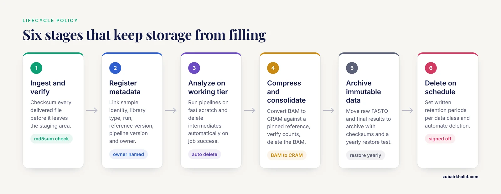
Capacity planning fails without a lifecycle policy, because storage fills with data that nobody will ever delete. A workable policy for bioinformatics data management has six stages.
- Ingest and verify. Compute a checksum on every delivered file before it leaves the staging area. A one-line habit catches silent transfer corruption that would otherwise poison a pipeline months later. An example invocation is
md5sum sample01_R1.fastq.gz > sample01_R1.fastq.gz.md5, verified again after any copy between tiers.
- Register metadata. Every dataset gets a record linking sample identity, library type, instrument run, reference genome version, pipeline version, and owner. Metadata is what makes an archive usable, and rebuilding it after the fact costs more than collecting it at ingest.
- Analyze on the working tier. All pipeline execution happens on fast scratch or parallel storage. Intermediate files get deleted on job success, automatically, by the pipeline itself, not by a well-meaning human weeks later.
- Compress and consolidate. At project close, convert BAM to CRAM against a pinned reference, verify read counts match, and delete the BAM. Consolidate project outputs into a versioned results bundle. At this point the durable holdings per genome drop substantially, which compounds across thousands of samples.
- Archive immutable data. Raw FASTQ and final results move to archive with checksums, metadata records, and a documented restore test at least annually. An archive that has never been restored is a hypothesis, not a backup.
- Delete on schedule. Define retention periods per data class in writing, get them signed off by data governance, and automate deletion. Duplicates from deliveries, ad hoc copies, and abandoned pilot projects should have named owners and expiry dates from day one.
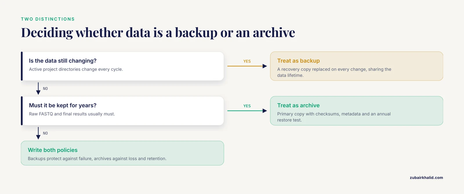
Two distinctions prevent most lifecycle confusion. A backup is a recovery copy that shares the data's lifetime and is replaced on every change. An archive is a primary copy of data you stopped changing, retained long-term. Conflating them produces either no recovery capability or unbounded growth. And a distinction that matters more every year is that AI pipelines add their own artifacts. Systems that link omics evidence with literature knowledge, such as OASIS, accumulate knowledge bases, benchmark results, and reusable procedural rules alongside the primary data they interrogate [4]. Decide now whether those artifacts are versioned products with retention policy or disposable scratch, before ad hoc decisions accumulate a third data estate.
Common Mistakes and Limitations
- Sizing for today instead of the curve. A purchase that meets current volume with no growth margin is obsolete on delivery. Always size against the three-year projection, not last year's actuals.
- Forgetting protection overhead. Teams that budget logical data and discover physical capacity needs only at provisioning time lose a factor of roughly two. Protection design belongs in the forecast, not the rack.
- Ignoring bandwidth. Buying capacity without matching input/output bandwidth creates a large, slow filesystem that throttles every pipeline. Working-set performance is a separate purchase from archival capacity.
- Confusing backup with archive. Backups protect against failure, archives protect against loss and satisfy retention. Each needs its own design, and neither substitutes for the other.
- Ignoring retrieval economics. Deep archive tiers charge for retrieval, and pipelines that accidentally read from archive can generate charges that dwarf storage costs. Keep archive reads behind explicit, human-triggered processes.
- Letting metadata lag the data. Data without sample identity, reference version, and pipeline provenance is reanalysis-proof ballast. Metadata capture is the cheapest capacity investment available because it determines whether old data is worth keeping at all.
- Treating staff as overhead. The UVRI experience demonstrates that human capacity, structured planning, and service management are what sustain infrastructure over years, and that underinvestment in people is the leading cause of abandoned systems [6].
- Assuming cloud or on-premises is a moral position. Both estates fail without governance and succeed with it. Choose by workload shape, skills, and compliance, and expect a mix.
- Planning for AI workloads as an afterthought. Healthcare AI deployment is growing exponentially, and genomics is a primary perception modality for these systems [3]. Feature tables, embeddings, model checkpoints, and benchmark outputs need the same lifecycle policy as sequencing reads.
Limitations. Every per-sample figure in this guide is a planning approximation, and real instruments, library kits, and pipelines vary. Treat the worked numbers as starting points for your own measurements, and re-baseline annually. Capacity plans are also institutional commitments, not mathematical outputs, so legal retention requirements, funding cycles, and partner agreements will modify the arithmetic. Finally, no storage plan substitutes for privacy governance on human genomic data, which remains an open ethical challenge across the field [1].
Frequently Asked Questions
How much storage do I need for one human whole genome?
Plan on roughly 100 GB of raw FASTQ, 40 to 50 GB as CRAM, and 5 to 10 GB of gVCF, which lands at 150 to 170 GB of durable holdings per genome before protection copies. Multiply by your annual sample count, apply a modest multiplier for intermediates during analysis, and double for replication or erasure coding.
Should I store BAM or CRAM files?
Store CRAM for anything you intend to keep more than a few months. CRAM stores reads as differences against a reference genome and typically cuts alignment storage roughly in half. Keep the reference genome version pinned alongside the CRAM so the files remain readable, and verify counts before deleting the original BAM.
How often should I re-forecast my capacity plan?
Re-forecast every six months against actual sequencing output and at least annually against the full five-step model. Also trigger an off-cycle review whenever a new instrument, assay modality such as single-cell or long-read, or a funded multiomic project enters the pipeline, because these change the per-sample footprint more than volume growth does.
Is cloud or on-premises better for genomics data storage?
Neither is universally better. On-premises parallel storage wins for daily pipeline throughput and data locality, cloud wins for elastic growth, durable archive, and collaborative access, and most mature programs run a hybrid that matches each tier to its workload. Decide by workload shape, in-house skills, and compliance obligations rather than by ideology.
What is the difference between backup and archive?
A backup is a recovery copy of data that is still changing, replaced on every cycle so you can restore after corruption or deletion. An archive is the primary copy of data you have stopped changing, retained for years with checksums and metadata. Raw FASTQ belongs in archive, while the active project directory needs backups, and treating one as the other causes both data loss and unbounded growth.
How do I plan capacity for AI and machine learning workloads?
Treat AI pipelines as a distinct data consumer with its own footprint, including training features, embeddings, model checkpoints, and benchmark results. Estimate their per-project volume the same way you estimate assay data, assign retention policy per artifact type, and keep the working training set on fast storage with the rest in warm or archive tiers.
Sources
- Transformative Applications and Innovations in Next-Generation Sequencing Data Analysis.
- The evolving role of genetic counselors in South Africa: A decade of growth.
- A comprehensive survey of AI agents in healthcare.
- OASIS, a self-evolving AI scientist that integrates omics data and literature knowledge for plant stress research.
- Identifying pleiotropic genes for backfat thickness and semen traits in pigs using GWAS summary data.
- A scalable HPC framework for bioinformatics in resource-limited settings: design principles, implementation, and sustainability from the UVRI experience.
- Decoding age-stratified clinical and molecular heterogeneity in male breast cancer through multiomic profiling.