How to Draw Genomic Ideograms in Python: A Practical Guide
By Dr. Zubair Khalid, DVM, MS, PhD ·

By the end of this guide you will be able to build a publication-quality genomic ideogram in Python: a simplified chromosome cartoon showing bands, the centromere, and labeled regions, with your own genes, variants, or copy-number segments overlaid on top. You will need a recent Python 3 installation, a terminal, roughly 50 MB of free disk space, and the cytoband coordinates for your genome build. Every command in this walkthrough runs on Linux, macOS, and Windows Subsystem for Linux.
Python has become a default language for bioinformatics visualization, and the ecosystem keeps producing domain-specific packages with dedicated plotting and diagnostic functions, from sequence-design evaluation to phylogenetics [1][2][3]. Ideograms are one of the few standard genome graphics with no single dominant Python library, which is exactly why this guide builds the core figure yourself and then shows where established libraries save time.
What a Genomic Ideogram Actually Shows
An ideogram is a schematic drawing of a chromosome. It compresses hundreds of millions of base pairs into a compact bar whose shading represents cytogenetic bands, the light and dark stripes visible when chromosomes are stained and viewed under a microscope, a technique known as G-banding. Standard ideogram elements include the following.
- The p arm (short arm) and q arm (long arm), separated by the centromere, the constricted region drawn as a distinct colored block, usually in the acen stain category.
- Telomeres, the chromosome ends.
- Bands named by position, for example 17q21.31 means chromosome 17, long arm, region 2, band 1, sub-band 31.
- Optional overlays: genes, GWAS loci, structural variants, or copy-number segments plotted at their base-pair coordinates.
The mapping from base pairs to bands comes from a cytoband file. You never have to derive band positions yourself. You download them, parse them, and draw them.
Choosing Your Drawing Strategy
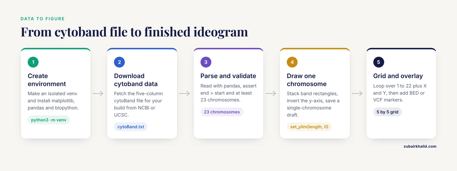
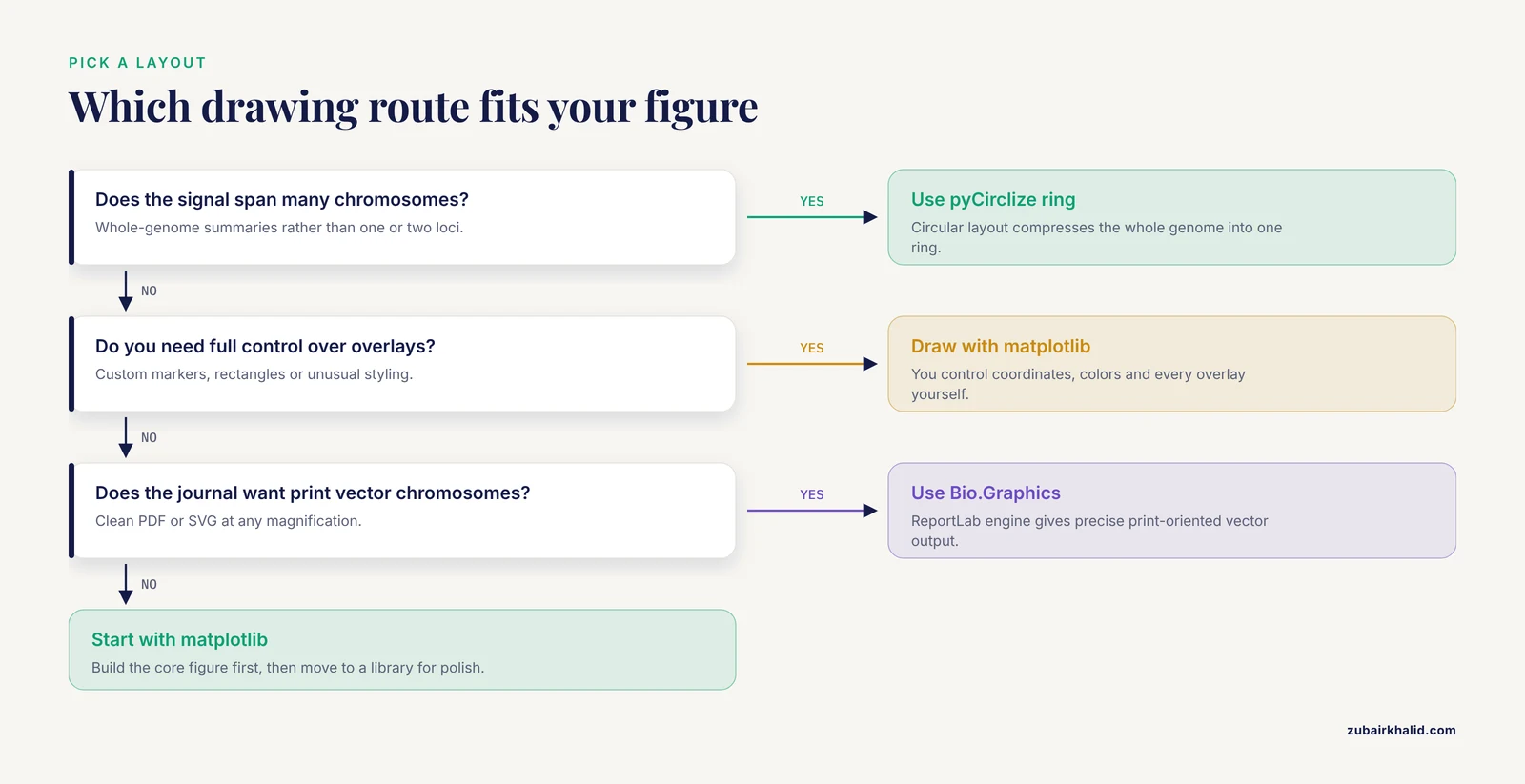
There are two viable strategies, and this guide teaches both.
- Draw the ideogram yourself with matplotlib, the standard Python plotting library. This gives you total control over coordinates, colors, and overlays, and it teaches you what an ideogram actually is.
- Use established drawing code for polish: Biopython provides chromosome diagram classes in its
Bio.Graphicsmodule, and pyCirclize produces circular (Circos-style) layouts.
A recent survey of the bioinformatics tooling literature shows the same pattern across subfields: specialized Python packages now handle visualization end to end, from phylogenomic trees with the ETE Toolkit to interactive workflow dashboards, and reproducibility through scripted execution is treated as a baseline requirement rather than a nicety [2][4][3]. Drawing your own ideogram with matplotlib fits that philosophy, because a script that reads a cytoband file and writes a figure is fully reproducible.
Step 1: Set Up a Clean Python Environment
Never install plotting libraries into your system Python. Create an isolated environment so versions are pinned and the figure can be regenerated years later.
python3 -m venv ~/venvs/ideogram
source ~/venvs/ideogram/bin/activate
pip install --upgrade pip
pip install matplotlib pandas biopython
To verify the install, open Python and check the versions:
import matplotlib, pandas, Bio
print(matplotlib.__version__, pandas.__version__, Bio.__version__)
Expected output is a line with three version numbers, for example 3.9.2 2.2.3 1.85.
Conda users can do the same thing with a channel-managed environment. Scientific Python packages are routinely packaged for conda-based distribution, and Bioconda in particular publishes packaged versions of bioinformatics tools such as scXMatch that you install with a single command [5]. The equivalent here is:
conda create -n ideogram python=3.11 matplotlib pandas biopython
conda activate ideogram
Containerize the environment if the figure must be regenerated on other machines. Fully containerized pipelines with Docker or Apptainer are now standard practice in published bioinformatics workflows precisely because they freeze the software versions that produced a given result [4]. A one-line Dockerfile starting from python:3.11-slim plus a pip install line is enough for this project.
Step 2: Get Cytoband Data
Two standard sources provide cytoband coordinates.
- NCBI distributes cytogenetic band files through its genome annotation FTP areas for each assembly, for example GRCh38 for the human genome.
- UCSC distributes the
cytoBand.txtfile for each human assembly through its downloads site.
The file is a five-column, tab-separated text file. The columns follow the UCSC table schema.
| Column | Content | Example |
|---|---|---|
| 1 | Chromosome name | chr17 |
| 2 | Band start position in bp | 19,900,000 style integer 19900000 |
| 3 | Band end position in bp | 20700000 |
| 4 | Band name | q21.31 |
| 5 | Stain class | gpos50 |
The stain class controls shading. The values you will encounter are gneg (light, negative G-banding), gpos25, gpos50, gpos75, and gpos100 (increasingly dark positive bands), acen (centromere), gvar (variable telomeric regions), and stalk (the stalk region of acrocentric chromosomes such as 13, 14, 15, 21, and 22). This staining scheme is standard cytogenetics, described in every human genetics textbook.
Download a file and inspect it:
head -5 cytoBand_hg38.txtExpected output looks like this (exact values depend on the build):
chr1	0	2300000	p36.33	gneg
chr1	2300000	5400000	p36.32	gpos25
chr1	5400000	7200000	p36.31	gneg
chr1	7200000	9200000	p36.23	gpos25
chr1	9200000	12700000	p36.22	gneg
Step 3: Parse the Cytoband File
Load the file with pandas, naming the columns explicitly because the file has no header.
import pandas as pd

COLS = ["chrom", "start", "end", "band", "stain"]
bands = pd.read_csv("cytoBand_hg38.txt", sep="\t", header=None, names=COLS)

# Basic sanity checks before drawing anything
assert (bands["end"] > bands["start"]).all(), "A band ends before it starts"
assert bands["chrom"].nunique() >= 23, "Fewer than 23 chromosomes found"

chrom_length = bands.groupby("chrom")["end"].max()
print(chrom_length.head())
Expected output:
chrom
chr1    248956422
chr2    242193529
chr3    198295559
chr4    190214555
chr5    181538259
These lengths are the assembly-specific chromosome sizes, and the exact numbers above match GRCh38, the current human reference assembly. If your numbers differ wildly, you are probably looking at a different build. Robust input and output handling for standard bioinformatics formats is a recurring design goal in modern Python frameworks, and it applies to your own scripts too: validate what you load before you draw it [3].
Step 4: Draw a Single-Chromosome Ideogram with matplotlib
This is the core of the guide. Each band becomes a filled rectangle, stacked vertically, with the chromosome drawn as a thin column. Short arms conventionally point up, so the y-axis is inverted so that position 0 sits at the top.
import numpy as np
import matplotlib.pyplot as plt
from matplotlib.patches import Rectangle

# Shading per stain class. Greys for gpos, white for gneg, lilac for acen.
STAIN_COLORS = {
    "gneg":    "#FFFFFF",
    "gpos25":  "#E0E0E0",
    "gpos50":  "#AAAAAA",
    "gpos75":  "#666666",
    "gpos100": "#2E2E2E",
    "acen":    "#C8A2C8",
    "gvar":    "#FFFFFF",
    "stalk":   "#9EC9E2",
}

def draw_ideogram(ax, bands, chrom, width=0.6, label_bands=True):
    sub = bands[bands["chrom"] == chrom].sort_values("start")
    if sub.empty:
        raise ValueError(f"No bands found for {chrom}. Check chromosome naming.")
    chrom_length = sub["end"].max()

    for _, row in sub.iterrows():
        color = STAIN_COLORS.get(row["stain"], "#FFFFFF")
        ax.add_patch(Rectangle(
            (0, row["start"]),
            width,
            row["end"] - row["start"],
            facecolor=color,
            edgecolor="black",
            linewidth=0.4,
        ))
        if label_bands and row["stain"] in ("gneg", "gpos50", "gpos75", "acen"):
            midpoint = (row["start"] + row["end"]) / 2
            ax.text(width + 0.06, midpoint, row["band"],
                    va="center", fontsize=7)

    ax.set_ylim(chrom_length, 0)          # p arm at top
    ax.set_xlim(-0.1, width + 1.4)
    ticks = np.linspace(0, chrom_length, 6)
    ax.set_yticks(ticks)
    ax.set_yticklabels([f"{t/1e6:,.0f}" for t in ticks])
    ax.set_ylabel(f"{chrom} position (Mb)")
    ax.set_xticks([])
    for spine in ax.spines.values():
        spine.set_visible(False)

fig, ax = plt.subplots(figsize=(3, 8))
draw_ideogram(ax, bands, "chr17")
fig.savefig("chr17_ideogram.png", dpi=300, bbox_inches="tight")
What you should see when you open chr17_ideogram.png: a narrow vertical column, mostly alternating light and grey stripes, with two lilac (acen) blocks roughly two-thirds of the way down marking the centromere of chromosome 17, band labels such as p13.1 and q21.33 printed to the right of the column, and a y-axis in megabases descending from 0 at the top.
The parameters that matter most here:
widthcontrols how thick the chromosome bar is in axis units. Keep it under 1.0 so label text does not collide.linewidth=0.4on each rectangle creates the thin borders that make bands readable at print size.set_ylim(chrom_length, 0)inverts the axis. Without it, the figure places the q arm on top, which readers of cytogenetics literature will find disorienting.fontsize=7on band labels. At 300 dpi this remains legible in a two-column journal figure.
If you are building a multi-panel figure that compares the same chromosomes across specimens, apply one consistent scale to every panel. Inconsistent per-panel scaling is a known pain point in comparative imaging visualization, and recent Python tools address it by enforcing shared scaling across specimens [6]. The same principle applies to ideograms: pick one axis convention and never mix scales within a figure.
Step 5: Draw a Full Karyotype Grid
A karyotype shows every chromosome in one figure, usually in a grid. The only new work is layout management.
ORDER = [f"{i}" for i in range(1, 23)] + ["X", "Y"]
normalized = bands.copy()
normalized["chrom"] = normalized["chrom"].str.replace("chr", "", regex=False)

ncols, nrows = 5, 5
fig, axes = plt.subplots(nrows, ncols, figsize=(11, 15))

for idx, chrom in enumerate(ORDER):
    ax = axes[idx // ncols][idx % ncols]
    try:
        draw_ideogram(ax, normalized, chrom, label_bands=(idx < 4))
    except ValueError:
        ax.set_visible(False)   # handles assemblies missing chrY

# Hide unused cells
for idx in range(len(ORDER), nrows * ncols):
    axes[idx // ncols][idx % ncols].set_visible(False)

fig.suptitle("Human karyotype (GRCh38)", fontsize=14)
fig.tight_layout()
fig.savefig("karyotype.png", dpi=300, bbox_inches="tight")
Expected result: chromosomes 1 through 22 plus X and Y arranged left to right and top to bottom, each drawn to its true relative length because the y-axis spans that chromosome's real base-pair range, with full band labels only on the leftmost column to keep the figure uncluttered.
The str.replace("chr", "", regex=False) line matters. Cytoband files from NCBI typically use plain 17 while UCSC uses chr17, and your overlay files may use either. Normalizing chromosome names at load time is one of those small steps that prevents an entire class of silent failures later. Modern toolkits treat consistent coordinate and identifier handling across data modalities as a first-class feature for exactly this reason [7].
Step 6: Overlay Your Own Data
An ideogram becomes scientifically useful when your data sits on it. The most common overlay formats are BED for regions and VCF or BED-like tables for point variants. This is also where Biopython earns its place in the pipeline, because it parses the standard sequence and annotation formats cleanly, as covered in any Biopython tutorial chapter on sequence input and output.
Reading gene locations from a BED file and marking them on the chromosome:
features = pd.read_csv(
    "genes.bed", sep="\t", header=None,
    names=["chrom", "start", "end", "name"],
)
features["chrom"] = features["chrom"].str.replace("chr", "", regex=False)

def draw_ideogram_with_hits(ax, bands, features, chrom, width=0.6):
    draw_ideogram(ax, bands, chrom, width=width, label_bands=True)
    hits = features[features["chrom"] == chrom]
    for _, f in hits.iterrows():
        midpoint = (f["start"] + f["end"]) / 2
        ax.plot([width + 0.5], [midpoint], marker=">",
                color="crimson", markersize=6)
        ax.text(width + 0.62, midpoint, f["name"],
                va="center", fontsize=7, color="crimson")

fig, ax = plt.subplots(figsize=(3, 8))
draw_ideogram_with_hits(ax, normalized, features, "17")
fig.savefig("chr17_with_genes.png", dpi=300, bbox_inches="tight")
Expected result: the chr17 ideogram with red arrow markers and gene names pointing at the bands that contain each gene from the BED file.
A caution about coordinates. BED uses a zero-based, half-open convention: start counts from base 0, and end excludes the final base. GFF and GTF use one-based, closed coordinates. Cytoband files follow the UCSC positional convention where the first base is position 0. If you mix conventions without converting, every overlay lands one base off, which is invisible for a 50 kb band but wrong for point variants. Verify placement against a known landmark, for example a gene whose cytogenetic band you know from the literature, before trusting the figure.
For association data, the same overlay logic applies. Published GWAS analysis pipelines implemented in Python routinely include genome-wide visualization as an explicit step, plotting refined signals back onto the genome before fine-mapping and downstream interpretation [8]. Plotting your top loci on a karyotype is a fast visual sanity check that hits cluster where the biology expects them, for example inside known immune loci for immune traits.
If your data lives in a different tool, interoperability is straightforward in principle. Modern bioinformatics infrastructure increasingly emphasizes cross-language and cross-package integration, for example R/Bioconductor infrastructure that integrates directly with third-party Python tools [9], and interoperable Python toolboxes designed to plug into larger analysis ecosystems [7]. Export your features as BED or TSV, normalize chromosome names, and overlay them with the code above.
Step 7: Circular Layouts with pyCirclize
A linear ideogram emphasizes one or a few chromosomes. A Circos-style circular layout shows the whole genome as a ring, which is useful when your signal spans many chromosomes. The Python package pyCirclize builds these figures directly from chromosome sizes.
pip install pycirclizefrom pycirclize import Circos
sizes = (chrom_length / 1e6).round().astype(int).to_dict() # size in Mb
circos = Circos(sizes, space=5)
for name, sector in circos.sectors.items():
track = sector.add_track((92, 100))
track.axis(fc="lightgrey", ec="black", lw=0.5)
track.text(name, r=105, size=8)
circos.savefig("genome_ring.png", dpi=300)Expected result: a ring of 24 grey arcs, one per chromosome, labeled at the outside, with free radial space inside each sector where you can plot heatmaps, scatter points, or links between chromosomes. The exact styling API has many options, so treat this snippet as a skeleton and build up tracks one at a time, saving after each addition so you can see what each track changed.
The circular-versus-linear tradeoff is a genuine design decision. Circular figures compress the whole genome but distort distance perception and make band labels hard to read. Linear ideograms scale poorly past a handful of chromosomes but are unambiguous. Reviewers of manuscripts containing both styles frequently ask for the other format, so generate both while the script is fresh.
Step 8: Vector Output with Biopython Bio.Graphics
For publication figures you want vector output (PDF, SVG, or EPS), which stays sharp at any magnification. matplotlib already produces vector formats, so fig.savefig("karyotype.pdf") is often sufficient. Biopython offers a second path through its Bio.Graphics module, which builds chromosome diagrams on the ReportLab drawing engine.
The relevant classes are BasicChromosome.Organism (the whole karyotype page), BasicChromosome.Chromosome (one chromosome, sized proportionally via its scale_num attribute), and BasicChromosome.ChromosomeSegment (one drawable chunk of the chromosome). A minimal single-chromosome example:
from reportlab.lib.units import cm
from Bio.Graphics import BasicChromosome

organism = BasicChromosome.Organism()
chrom = BasicChromosome.Chromosome("17")
chrom.scale_num = int(chrom_length["chr17"])  # longest chr length, for scaling

segment = BasicChromosome.ChromosomeSegment()
chrom.add(segment)
organism.add(chrom)
organism.draw("chr17_biopython.pdf", "Chromosome 17")
The full worked karyotype script, including telomere segments and per-band coloring, is in the chromosome-diagram chapter of the official Biopython tutorial, which is the authoritative reference for this API. Use matplotlib for exploratory figures and overlays, and reach for Bio.Graphics when you want ReportLab's precise, print-oriented vector layout.
One more option worth knowing for gene-scale maps: DNA Features Viewer draws annotated feature diagrams from simple GraphicFeature objects or parsed GenBank records, which pairs naturally with Biopython's Bio.SeqIO parsing:
from Bio import SeqIO

record = SeqIO.read("plasmid.gb", "genbank")
genes = [
    (int(f.location.start), int(f.location.end))
    for f in record.features if f.type == "gene"
]
That reads every gene feature from a GenBank file with known, documented Biopython behavior, and you can feed the coordinates into any of the drawing approaches above.
Tool Comparison
| Tool | Layout style | Typical input | Output formats | Best used for |
|---|---|---|---|---|
| matplotlib (this guide) | Linear karyotype | Cytoband TSV plus BED/TSV overlays | PNG, PDF, SVG | Full control, teaching, custom overlays |
Biopython Bio.Graphics | Vertical chromosome diagrams | Band coordinates, feature lists | PDF, SVG via ReportLab | Print-quality vector figures |
| pyCirclize | Circular ring | Chromosome sizes, track data | PNG, PDF | Genome-wide signal summaries |
| DNA Features Viewer | Linear feature maps | GenBank, GFF, GraphicFeature lists | PNG, SVG | Gene and plasmid level maps |
| pyGenomeTracks | Stacked genomic tracks | Track config file, BED, bigWig | PNG, PDF | Data tracks aligned under a coordinate axis |
Rule of thumb: matplotlib when you need something the libraries do not already draw, pyCirclize for whole-genome rings, Bio.Graphics when the journal wants clean vector chromosomes, and DNA Features Viewer when the unit of display is the gene rather than the chromosome.
Genomic Ideogram Python Tips for Better Figures
Pick one resolution and stay at it. An ideogram at band resolution is a summary graphic. If the scientific claim depends on features smaller than a band, switch to a zoomed track view such as pyGenomeTracks for the region in question rather than forcing the ideogram to carry detail it cannot show.
Normalize chromosome names once, centrally. Decide on chr17 or 17 at load time, strip or add prefixes in one function, and route every input through it. Name mismatches between the cytoband file and overlay files are the single most common cause of a silently empty figure.
Test with one chromosome before rendering 24. Iterate on chr1 or chr17 at high dpi, get the styling right, then run the loop over the full order list. Saving intermediate drafts after each change lets you attribute visual problems to the change that introduced them, a habit that interactive exploration tools in recent Python bioinformatics packages formalize deliberately [1][4].
Keep shading monotonic. Map gneg through gpos100 to a strictly increasing darkness scale, and use one distinct hue for acen. Readers interpret ideograms by stain intensity, so arbitrary colors break the grammar of the figure.
Use colorblind-safe overlays. Red markers on grey bands are readable, but red plus green overlays are not. Verify with a colorblindness simulator before submission.
Batch-compare with identical axes. When comparing ideograms across individuals or assemblies, fix the scaling rules in the script rather than letting each panel autoscale. Shared-scaling design is the central lesson of recent cross-specimen visualization tooling in Python [6], and it transfers directly.
Script the whole figure, including data download. Modern reproducibility practice in the field pushes visualization into scripted, containerized workflows rather than manual GUI steps, whether the tool exposes Python, R, or command-line interfaces [4][10]. Your ideogram script should regenerate the figure from raw files with one command.
Common Mistakes and Limitations
Mixing genome builds. Coordinates from GRCh37 (hg19) plotted on a GRCh38 (hg38) ideogram can be off by thousands to millions of bases depending on the region, because assemblies differ in gap placement and sequence. Convert with a proper liftOver-style chain file, never by eye, and record the build in the figure caption.
Ignoring coordinate conventions. As described in Step 6, BED is zero-based half-open while GFF is one-based closed. A point variant annotated one-based and plotted as if zero-based shifts by one base, which corrupts precise overlays. Convert once, in the loader, with a comment explaining which convention each file uses.
Chromosome naming mismatches. 1 versus chr1 produces an empty filtered DataFrame rather than an error. Add the assertion shown in Step 3, and check bands["chrom"].unique() when a figure comes out blank.
Forgetting the axis inversion. Without set_ylim(length, 0), the q arm appears above the p arm. Any cytogeneticist reviewing the figure will notice immediately.
Assuming the centromere is one block. In real cytoband files the centromere is represented by two adjacent acen bands, one on the p side and one on the q side. If your centromere marker logic assumes a single row, it will fire twice or in the wrong place. Group or merge adjacent acen rows if you need a single marker.
Overplotting. Thousands of overlay points on a band-resolution graphic turns the figure into noise. Bin or thin the data, or move dense layers to a companion track figure.
Treating the ideogram as data. An ideogram is a schematic. Band boundaries are cytogenetic landmarks, not sequence-precise annotations, and the mapping between bands and base pairs is approximate at band scale. Do not compute statistics off ideogram coordinates when sequence coordinates exist.
Label collisions at small figure sizes. Band labels at fontsize 7 overlap on short chromosomes. Turn labels off for grid layouts except a reference column, as in Step 5.
A final limitation: a drawn ideogram communicates position, not mechanism. It is a display layer. The claims your figure supports come from the analysis upstream of it, and the figure should be labeled with the genome build and data sources so the display cannot be mistaken for the evidence.
Next Steps
Once the basic pipeline runs, natural extensions are copy-number segments drawn as colored rectangles spanning genomic intervals, structural variants drawn as arcs or links between band positions (pyCirclize handles inter-sector links well), and a small configuration file that drives the script so colleagues can regenerate figures for different assemblies without touching code. If you publish the script, containerize it as described in Step 1 so the figure and its exact software versions travel together, mirroring the reproducibility patterns that current bioinformatics workflow papers treat as standard [4][10].
Frequently Asked Questions
What is a genomic ideogram?
A genomic ideogram is a schematic chromosome diagram in which shading represents cytogenetic bands, the centromere is shown as a distinct block, and genomic positions are mapped from base pairs onto the simplified chromosome cartoon. It is the standard chromosome graphic used in cytogenetics and genome-wide studies.
Which Python library is best for drawing genomic ideograms?
There is no single dominant library, so the best choice depends on the figure. matplotlib gives full control for linear karyotypes, Biopython's Bio.Graphics provides polished vector chromosome diagrams, and pyCirclize produces circular whole-genome layouts. This guide's matplotlib approach is the most flexible starting point.
Where do I get cytoband coordinate data?
Cytoband files are distributed by NCBI through each assembly's genome annotation FTP area and by UCSC as cytoBand.txt files for each human genome build. The files are five-column, tab-separated text listing chromosome, start, end, band name, and stain class.
Can I overlay my own data such as VCF or BED files on an ideogram?
Yes. Convert your features to a table with chromosome, start, and end columns, normalize chromosome names against the cytoband file, and plot markers or rectangles at the matching coordinates in the same axis system as the ideogram.
Why does my ideogram look upside down or mirrored?
The standard convention places the p arm (short arm) at the top, which requires an inverted y-axis with position 0 at the top. If your figure shows the q arm on top, you skipped the set_ylim(length, 0) inversion step.
Do I need Biopython or is matplotlib enough?
Matplotlib alone is enough to draw ideograms from cytoband files. Biopython is worth adding when you parse GenBank, FASTA, or other standard formats, or when you want the ReportLab-based vector chromosome diagrams in Bio.Graphics.
How do I handle different genome builds like hg19 and hg38?
Choose one build for the ideogram and every overlay, download cytoband data for that same build, and convert any data from another build using coordinate liftOver-style chain files. Never plot coordinates from one build directly onto an ideogram of another.
Can I save ideograms as vector files for publication?
Yes. matplotlib exports PDF and SVG directly through savefig, and Biopython's Bio.Graphics writes PDF and SVG through ReportLab. Vector output keeps bands and labels sharp at any print size.
Sources
- seqme: a Python library for evaluating biological sequence design from generative models.
- An Integrated Ecosystem for Analysis and Visualization of Large-Scale Phylogenomic Data Combining ETE Toolkit, TreeProfiler, and PhyloCloud for Scalable Phylogenomic Analysis.
- PhyloZoo: a unified framework for phylogenetic network analysis in Python.
- PerSeqPIPE: Nextflow workflow for per-sequence analysis of small RNA-sequencing data.
- Quantifying distribution shifts in single-cell data with scXMatch.
- ScaleBarOn and Muad'Data: simple Python tools for elemental imaging data visualization and comparative scaling.
- Spatialproteomics: an interoperable toolbox for analyzing highly multiplexed fluorescence image data.
- Large-Scale Data Analysis of Post-Traumatic Stress Disorder (PTSD) Through GWAS Fine-Mapping and Systems Biology.
- An Open Infrastructure for Mass Spectrometry Data in R.
- Fast-nnt: fast, reproducible, and scalable neighbour network analysis in R, Python, and CLI.