Reducucing Cloud Storage Costs for Genomic Data
By Dr. Zubair Khalid, DVM, MS, PhD ·
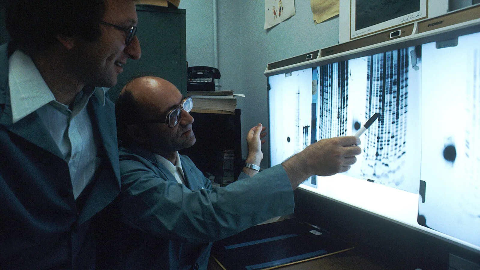
Sequencing output grows faster than most budgets. High throughput sequencing technologies and the falling cost of sequencing have driven exponential growth in stored sequence data, and that growth creates concrete challenges for storage, retrieval, and transmission [1]. A single sequencing core can generate tens of terabytes per month, and most of it sits untouched in expensive storage tiers while the lab moves on to the next run.
By the end of this article you will be able to inventory your cloud storage footprint, convert alignment files to a smaller format without losing data, compress raw reads with the right tools, apply lifecycle policies that move cold data into cheaper storage classes automatically, and adopt compute-to-data workflows that keep both storage and transfer costs down. The walkthrough uses Amazon S3 with the AWS CLI because aws genomics workloads dominate cloud bioinformatics practice, but the same principles apply on Google Cloud and Azure. Published comparisons show the structure of the cost problem is consistent across providers, so the strategy transfers [2][3].
To follow the walkthrough you need:
- The AWS CLI, version 2.x, installed and configured with credentials for an account that owns the buckets you want to optimize (
aws configuresets this up) samtoolsandhtslibversion 1.15 or later for alignment and FASTQ work- A reference genome FASTA and its
.faiindex for CRAM encoding - A spreadsheet or notebook for the cost baseline calculation in Step 1
Why Genomic Data Storage Bills Balloon
Three forces push genomic storage costs up. First, volume. NGS data are generated more rapidly than they can be analyzed, which means raw reads pile up faster than pipelines consume them [4]. A 30x human whole genome produces roughly 100 GB of FASTQ, and a population study with hundreds of samples multiplies that quickly.
Second, wrong storage classes. Cloud providers charge different rates depending on how quickly data can be retrieved. Most laboratories keep everything in the fastest, most expensive class by default, including year-old alignment files nobody has opened since the paper was submitted.
Third, redundant intermediates. Workflow systems make it easy to keep every intermediate file, and pipeline authors often leave SAM files, unsorted BAMs, temporary index files, and duplicate FASTQs behind. A systematic benchmark of cloud whole genome analysis found that strategic batching of individual genomes and efficient cluster resource configuration are what separate a cost-effective pipeline from an expensive one, and the same attention to detail applies to what gets written to storage in the first place [5].
Big data reviews in health care rank storage and transfer costs among the top challenges alongside data structure and governance, so this is a recognized infrastructure problem, not a sign that your lab is doing something unusual [6].
Know Your Data Before You Change Anything
Genomic data falls into a few access patterns, and each one points to a different cost strategy.
Hot data. Files a running pipeline reads this week. Active alignments, VCFs under analysis, references and indexes. Keep these in the fastest storage class. The cost lever here is not the storage class, it is file format and deleting intermediates.
Warm data. Published results, reference-backed BAM or CRAM files you might re-query occasionally. These belong in a cheaper infrequent-access class that still allows immediate retrieval.
Cold data. Raw reads and final deliverables that must be retained for years, often for grant or regulatory reasons. These belong in archive classes, where retrieval takes minutes to hours but per-TB storage cost drops dramatically.
Transfer-heavy data. Files that get pulled down repeatedly, or that sit in one cloud while compute runs in another. Transfer costs are a storage-adjacent expense that workflow design can eliminate, as the compute-to-data section explains.
Write down which categories exist in your buckets and roughly what fraction of total bytes each represents. Every step that follows depends on this picture.
A Step-by-Step Approach to Genomic Data Storage Cost Reduction
This walkthrough moves from measurement to compression to automation. Run each step on a test bucket or a small prefix before applying it to production data.
Step 1: Inventory and Cost Baseline
You cannot reduce what you have not measured. Get an accurate object count and total size for each prefix:
aws s3 ls s3://my-lab-genomics/ --recursive --summarize --human-readable | tail -5Expected output looks like this:
2026-09-14 11:22:03   98.4 GiB runs/2026-08/A001/alignments/A001.bam
2026-09-14 11:26:41  102.1 GiB runs/2026-08/A001/alignments/A001.bai
2026-10-02 09:41:12   95.7 GiB runs/2026-09/A002/alignments/A002.bam
...
  Total Objects: 48211
  Total Size: 312.4 GiB
For large buckets, this listing is slow. Use a CloudWatch storage metrics query or the provider's inventory report instead of walking millions of objects.
Now build the baseline formula. Cloud object storage bills three components:
Monthly cost = (TB stored x per-TB-month rate for the storage class)
             + (GB retrieved x retrieval rate, archive classes only)
             + (number of PUT/GET requests x per-request rate)
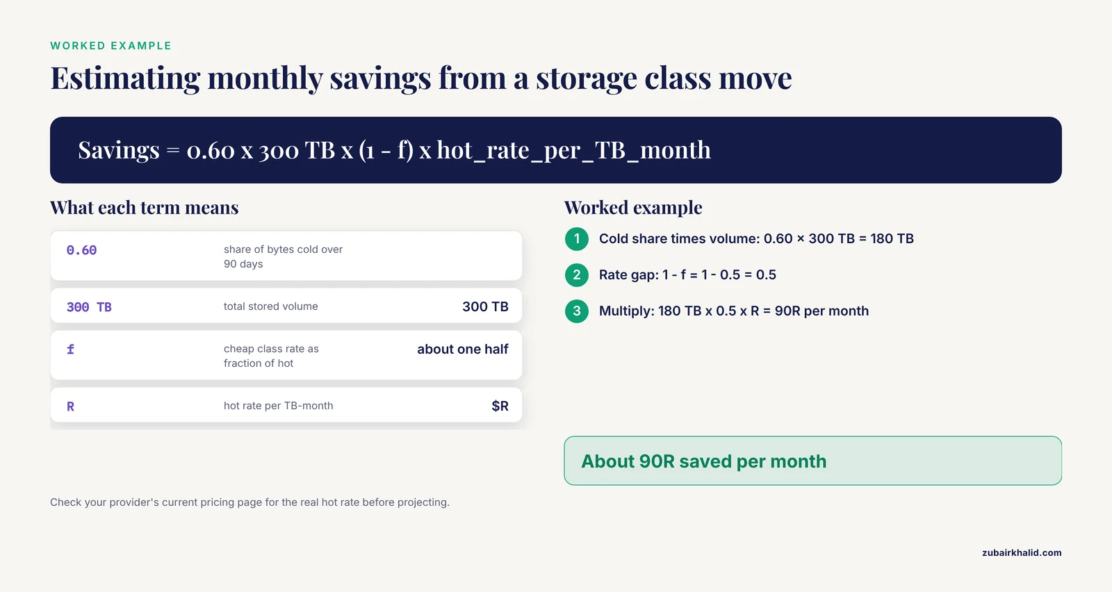
Substitute your provider's current listed rates for each variable. For a concrete worked example with symbolic rates, suppose you store 300 TB, of which 70 percent sits in the most expensive class, and 60 percent of total bytes have not been accessed in over 90 days. If a cheaper infrequent-access class costs a fraction f of the hot class rate, moving that 60 percent saves:
Savings = 0.60 x 300 TB x (1 - f) x hot_rate_per_TB_monthIf f is roughly one half and the hot rate is $R per TB-month, savings equal about 90R per month, or more than a terabyte-scale annual figure once multiplied out. The exact arithmetic depends on your provider's current pricing page, which you should check directly, but the formula and the access-pattern split are the part you control.
Record the baseline in your notebook. Every later step should shrink one of its terms.
Step 2: Convert BAM to CRAM
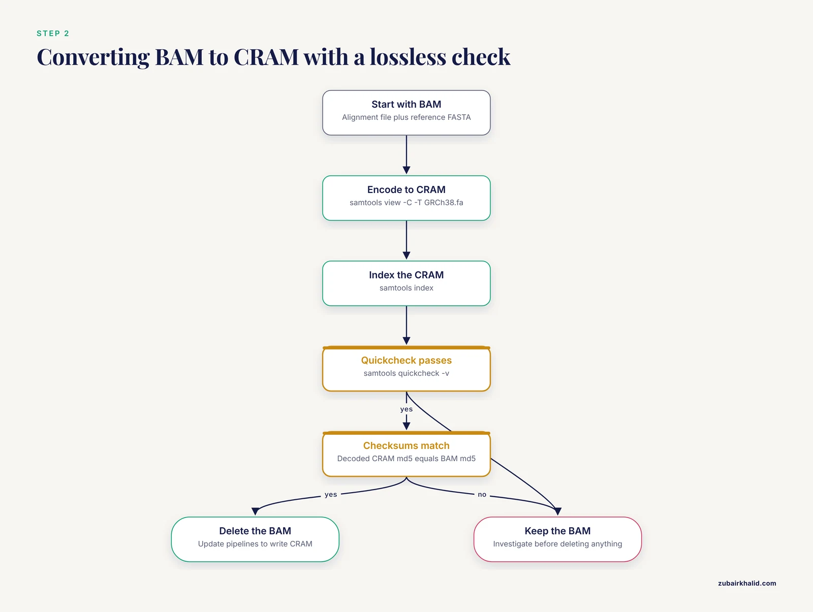
CRAM is the reference-based compression format for alignments in the HTS standards family. It achieves much smaller files than BAM because it stores reads as differences from a supplied reference rather than as full sequences, a strategy that reflects the broader division of genomic compressors into referential and reference-free approaches described in the compression literature [1]. CRAM is the single biggest format-level win most aws genomics pipelines leave on the table.
Convert with samtools:
samtools view -C -T GRCh38.fa \
  -o runs/2026-08/A001/alignments/A001.cram \
  runs/2026-08/A001/alignments/A001.bam

samtools index runs/2026-08/A001/alignments/A001.cram
The key parameters:
-Cselects CRAM output-T GRCh38.fanames the reference FASTA. Omitting it forces CRAM to embed reference stretches or fall back to lossy behavior depending on your options, so always pass it explicitly-m(for example-m 512M) tunes CRAM writer memory if you run on a small instance-output-fmt-option no_ref=1stores the file without reference dependence. This increases size but makes the CRAM self-contained. Use it only when you cannot guarantee the reference will remain available
Verify the conversion before deleting the BAM. samtools quickcheck confirms structural integrity:
samtools quickcheck -v runs/2026-08/A001/alignments/A001.cram && echo OKThen confirm data equality by comparing the decoded CRAM against the original BAM:
samtools view runs/2026-08/A001/alignments/A001.cram -T GRCh38.fa \
  | md5sum
samtools view runs/2026-08/A001/alignments/A001.bam | md5sum
Both checksums must match for a lossless round trip. The size gain depends on how well the reads match the reference. Reads aligned to a closely related reference compress far better than divergent reads, so run the comparison on one sample and record your own ratio before converting everything.
Once every CRAM verifies, delete the BAM copies and update pipeline defaults so future runs write CRAM directly.
Step 3: Compress FASTQ the Right Way
Raw reads are usually stored as FASTQ compressed with gzip, and plain gzip is often the wrong tool. The block-based gzip implementation bgzip produces files that are both smaller and indexable, which matters because random access to compressed genomic data is a recurring requirement in downstream tools:
bgzip -@ 8 -c sample_R1.fastq > sample_R1.fastq.gz
bgzip -@ 8 -c sample_R2.fastq > sample_R2.fastq.gz
-@ 8 uses eight compression threads. The resulting file remains readable by every tool that reads gzip, including samtools, cutadapt, and aligners, so there is no compatibility penalty.
For deeper savings, purpose-built FASTQ compressors exist. WBFQC, a lossless non-reference-based FastQ compressor, splits the data into homogeneous streams and applies a tuned algorithm to each, outperforming other state-of-the-art approaches in compression ratio and in compression and decompression time, while adding random access over the compressed data [4]. The general lesson from the compression literature is that specialized genomic compressors beat general-purpose ones, and that the choice between referential and reference-free methods depends on whether you can guarantee reference availability and can tolerate the tighter coupling that referential formats create [1].
Mass spectrometry data illustrate the same principle in another omics domain. MassComp, a lossless compressor for mass spectrometry files, reduced the numerical m/z-intensity data by 46 percent on average and up to 89 percent, achieved 59 percent reduction across whole repository files, and beat gzip by more than 27 percent on average [7]. If your lab also stores proteomics output, that result argues for auditing every stored omics data type, not just sequences.
Whatever compressor you choose, verify losslessness by decompressing and re-checksumming:
gunzip -c sample_R1.fastq.gz | md5sum
gunzip -c sample_R1_original.fastq | md5sum
Step 4: Apply Lifecycle Policies
A lifecycle policy tells the object store to transition objects between storage classes or delete them automatically based on age and tags. This is the highest-leverage automation for genomic data storage cost reduction because it acts on everything, including objects uploaded by scripts nobody remembers writing.
First, tag data by category during pipeline runs. Then apply a policy. Create lifecycle.json:
{
  "Rules": [
    {
      "ID": "intermediates-expire",
      "Filter": {"Tag": {"Key": "data-class", "Value": "intermediate"}},
      "Status": "Enabled",
      "Expiration": {"Days": 14}
    },
    {
      "ID": "warm-to-cold",
      "Filter": {"Tag": {"Key": "data-class", "Value": "keep"}},
      "Status": "Enabled",
      "Transitions": [
        {"Days": 30,  "StorageClass": "STANDARD_IA"},
        {"Days": 180, "StorageClass": "DEEP_ARCHIVE"}
      ]
    }
  ]
}
Apply it:
aws s3api put-bucket-lifecycle-configuration \
  --bucket my-lab-genomics \
  --lifecycle-configuration file://lifecycle.json
Then confirm the policy took effect:
aws s3api get-bucket-lifecycle-configuration --bucket my-lab-genomicsExpected output echoes both rules with their IDs and status.
The parameters that matter:
- Expiration Days deletes objects. Set it only on prefixes and tags you are certain are disposable. Intermediates such as unsorted SAM files and per-chunk work directories are good candidates. Final deliverables are not.
- Transitions Days controls when objects move to cheaper classes. The right intervals come from your access logs. Objects you have not touched in 30 days rarely become hot again.
- Tag filters scope each rule. A bucket-wide rule that transitions active pipeline scratch data to an archive class will cause retrieval stalls and retrieval fees, which is worse than the bill you were trying to fix.
Tag objects at upload time so the policy can classify them:
aws s3 cp intermediate.bai s3://my-lab-genomics/tmp/ \
  --metadata-directive COPY \
  --tagging "data-class=intermediate"
Step 5: Delete Duplicates and Dead Intermediates
Most buckets contain megabytes of the same reads stored three times. Find large objects and sort by size:
aws s3 ls s3://my-lab-genomics/ --recursive --human-readable \
  | grep -iE "\.(bam|sam|fastq|cram)$" | sort -k3 -h -r | head -30
Common duplicates to hunt for:
- Original FASTQ plus an identical re-uploaded copy under a different prefix
- BAM files that already exist as verified CRAM
.samintermediates from pipeline runs that were never converted to BAM- Per-chunk BAM shards from parallel variant calling that were merged and never removed
- Old index files (
.bai,.fai,.dict) for objects that no longer exist
Delete deliberately, by listing the exact objects:
aws s3 rm s3://my-lab-genomics/runs/2025-04/A001/tmp/A001.chunk12.samEnable bucket versioning review afterward. Versioning silently retains prior object versions, which means an "deleted" BAM may still be billed unless a version-expiration rule is in place. Add a noncurrent-version expiration rule to the lifecycle configuration from Step 4.
Step 6: Verify Storage Class Migration
Lifecycle transitions are asynchronous and can take up to a day or more per transition, depending on the class. Check a sample object:
aws s3api head-object \
  --bucket my-lab-genomics \
  --key runs/2026-08/A001/alignments/A001.cram \
  --query "[StorageClass, LastModified]"
Expected output shows the new class:
[
    "STANDARD_IA",
    "2026-08-14T11:22:03+00:00"
]
Objects still marked STANDARD after the transition window has passed indicate a policy filter that did not match. The most common cause is a tag key or value typo in the JSON rule.
Step 7: Adopt Compute-to-Data Workflows
Storage cost reduction eventually runs into a floor, and the next savings come from moving compute to the data instead of data to the compute. The paradigm is explicit in recent mega-biobank work. A fine-mapping analysis of the UK Biobank whole genome sequencing dataset on that cohort's cloud Research Analysis Platform demonstrated a 44 percent cost reduction and a 94 percent speedup through compute architecture optimization, aligning with the shift toward bringing compute to data [8]. Distributed, cloud-native analysis engines push in the same direction. A cloud-native distributed pileup implementation that partitioned alignments carefully and avoided costly data exchange between nodes ran up to 6.5 times faster with up to 2 times less memory than other state-of-the-art distributed tools, producing a substantial cloud cost reduction, and deploys on managed Kubernetes and Hadoop services available in public clouds [9].
The practical rules that follow from this work:
- Never download whole-genome files to a laptop or an on-premises server to analyze them. Run the analysis on the cloud platform where the data lives, using tools that read directly from object storage.
- Choose analysis tools designed for cloud object storage rather than for local filesystems. Spark-based frameworks such as Hail, used in comparative cloud cost evaluations of genome-wide association studies, are designed for exactly this pattern [2].
- When data must move between providers, use a high-speed transfer layer. The Closha workflow system paired its pipeline engine with KoDS, a data transmission solution reporting file transfer speeds up to 10 times that of normal approaches [10]. Slow transfers cost both egress fees and compute idle time.
Storage Classes Compared
The table below summarizes the storage class strategy. Retrieval behavior and relative cost relationships are standard, documented characteristics of cloud object storage. Check your provider's pricing page for current rates.
| Storage class | Retrieval latency | Relative storage cost | Retrieval fees | Use for |
|---|---|---|---|---|
| Hot (S3 Standard class) | Immediate | Highest | None | Active pipeline inputs, current run outputs, references and indexes |
| Infrequent access (S3 Standard-IA class) | Immediate | Lower | Per-GB retrieval | Published results, verified CRAM queried a few times per year |
| Archive with instant retrieval (S3 Glacier Instant Retrieval class) | Immediate | Lower still | Per-GB retrieval | Cold data still occasionally spot-checked |
| Flexible archive (S3 Glacier Flexible Retrieval class) | Minutes to hours | Low | Per-GB retrieval | Raw reads retained for reproducibility, rarely read |
| Deep archive (S3 Glacier Deep Archive class) | Hours | Lowest | Per-GB retrieval, bulk restore | Regulatory retention, raw reads and final deliverables you expect never to re-read |
Two behaviors deserve attention. First, archive-class objects must be restored before tools can read them, and restore jobs carry their own fees and wait times. Second, early-deletion minimums apply to most archive classes, so a lifecycle policy that archives an object for a week and then deletes it can cost more than keeping it in a hot class.
Compute Choices That Change the Storage Bill
Compute decisions and storage costs are coupled in both directions. Here are the couplings that matter, with the published evidence for each.
Spot and preemptible capacity. Discounted interruptible instances slash compute cost, and they change storage behavior too, because jobs that die mid-run leave partial outputs that must be cleaned up. Aether uses linear programming to optimally bid on and deploy combinations of underutilized cloud computing resources, simultaneously minimizing data analysis cost while easing the transition from existing HPC pipelines [11]. MC-GenomeKey extends this across providers, supporting Amazon, Google, and Azure clouds as well as any OpenStack-based platform, and explicitly supports scenarios that combine Amazon spot instances with resources from other clouds [3]. The design consequence for storage is simple. Spot-aware pipelines should write outputs atomically at job completion, not incrementally, so an interrupted run does not leave orphaned partial files billing you for years.
Strategic batching. The GenomeKey benchmark of cloud whole genome analysis showed that how you batch individual genomes and how you configure cluster resources determine both speed and cost at clinical scale [5]. Over-parallelizing writes thousands of tiny output files, and object storage bills per-request costs that scale with object count, not just bytes. Batch sensibly and object counts stay manageable.
Multi-cloud portability. Because the cost structure of genome-wide association studies proved consistent across Google Cloud Platform and Amazon Web Services when researchers compared Spark and Hail configurations [2], and because MC-GenomeKey demonstrated executable workflows spanning multiple commercial providers simultaneously [3], you have genuine leverage when negotiating storage and compute pricing. Pricing competition among cloud providers is itself cited as a resource for cost-effective clinical genomics services [3].
Workflow systems that manage resources for you. Closha provides drag-and-drop multi-step pipelines, imports Galaxy pipelines, and mixes traditional tools with MapReduce-based analysis in a single workflow [10]. COSMOS, the engine behind GenomeKey, implements complex workflows making optimal use of high-performance compute clusters [5]. Workflow systems centralize the output-writing decisions that determine your bucket's growth rate, which makes lifecycle tagging consistent across the whole lab.
Purpose-built distributed tools. Specialized engines also change the storage equation. HSRA extends a spliced read aligner for RNA-seq data to distributed memory systems through the MapReduce model on Hadoop clusters [12]. ConvCGP compresses genome-wide polymorphism data into a compact latent representation for prediction, explicitly reducing storage needs and computational load in agronomic genomics [13]. The common thread is that algorithm design and storage cost are linked, and tools designed for compressed or partitioned representations cost less to store and run.
At the extreme end of cost engineering, one project concluded that owning hardware beats renting. atSNPInfrastructure explored a database storage engine housing up to 307 billion SNPs for online access, evaluated database storage engines against constraints including dataset size, information gain, cost, and hardware, and built physical infrastructure whose final costs it compared against a major cloud provider [14]. The lesson is not that every lab should buy servers. The lesson is that at very large, very query-stable workloads, the cloud-versus-owned comparison is empirical, and you should run it for your own access pattern before assuming either answer.
Specialized Genomic Compression Beyond gzip
Two families of genomic compression are worth knowing by name, because choosing between them shapes your reference management obligations.
Reference-free compressors encode sequence data without requiring a reference genome. They are self-contained, simpler to archive, and safer for long-term regulatory retention, but they achieve smaller gains for resequencing data. WBFQC is an example, a lossless, non-reference-based FastQ compressor that streams data into homogeneous partitions and compresses each with an appropriate algorithm, while retaining random access into the compressed data [4].
Referential compressors store reads as differences from a reference. CRAM is the standard implementation, and the compression literature classifies this as one of the two fundamental strategies. Referential methods achieve the best ratios when reads closely match the reference, but they bind the archive to reference availability. If the reference is lost or replaced, decoding becomes harder. Keep the reference FASTA and its index in the same bucket and the same lifecycle policy as the CRAMs that depend on it, and record the reference checksum in your metadata.
The review literature on DNA sequence data compression documents this landscape comprehensively, categorizing methods and comparing their performance, and highlights open challenges that remain active research areas [1]. For a laboratory, the operational takeaway is narrower. Use CRAM for alignments with a well-managed reference, use bgzip for FASTQ that downstream tools must read directly, and evaluate specialized compressors only for data types where storage volume justifies the added tooling.
Common Mistakes and Limitations
Converting to CRAM without a reference management plan. CRAM reads depend on the reference used at encode time. Labs convert to CRAM, delete the reference, then discover a year later that the files cannot be decoded reliably. Store the reference alongside the CRAMs and record its checksum. If you cannot commit to reference custody, use no_ref=1 CRAM or stay with BAM and take your savings elsewhere.
Archiving data a pipeline still reads. A lifecycle rule that transitions active scratch prefixes into archive classes creates retrieval fees and multi-hour restore delays. The fix is tagging discipline, not aggressive global rules. Scope every rule by tag or prefix.
Deleting intermediates that are actually deliverables. Some intermediates, such as per-sample gVCFs in joint genotyping projects, are required inputs to future analyses. Classify before you expire. The 14-day expiration rule belongs on chunk-level SAM shards, not on gVCFs.
Ignoring object count. Billing includes per-request and per-object overheads on some classes. A pipeline that writes millions of tiny shard files can cost more in request fees than the bytes cost in storage. Batch outputs, as the GenomeKey work demonstrated.
Trusting checksums you never computed. Verify CRAM round trips with samtools quickcheck and md5 comparison before deleting the source BAM, as shown in Step 2. A truncated upload often produces a file with no valid BGZF end-of-file marker, which samtools quickcheck catches.
Treating egress as free. Downloading terabytes out of a cloud provider costs more per GB than storing them for a month in most configurations. Every download-first workflow is a storage-plus-transfer cost problem. Compute-to-data designs address this directly.
Assuming compression ratios transfer between data types. A 50 percent CRAM gain on human WGS tells you nothing about your metagenomic or RNA-seq data. Measure on your own samples before projecting savings.
Forgetting versioning and incomplete uploads. Aborted multipart uploads leave orphaned parts that bill silently. Configure incomplete multipart upload expiration in the lifecycle policy, and set noncurrent-version expiration if versioning is enabled.
Expecting identical economics on every provider. The comparative evidence shows speed-cost trade-offs were consistent across Google Cloud and AWS for GWAS workloads [2], but consistent structure is not identical pricing. Re-run the Step 1 baseline on each provider you use.
Overstating what format choice alone can do. Format conversion and compression reduce the storage term of the cost formula. They do nothing for transfer fees, request fees, or compute waste. The published cost reductions of 44 percent in mega-biobank analysis came from compute architecture optimization, not file formats alone [8].
Frequently Asked Questions
Does converting BAM to CRAM lose any data?
No. CRAM with the reference supplied is a lossless format under default settings, and the verification procedure in Step 2, comparing decoded output checksums against the original BAM, proves it for your own files. Only non-default options that discard information, such as storing without the reference in constrained modes or selectively dropping tags, change that, and you should never enable those options for archival data.
What is the fastest way to start reducing cloud storage costs for genomic data?
Delete dead intermediates and apply a tagged lifecycle policy. Both act immediately on data you already have, require no pipeline changes, and typically address the majority of wasted spend, because most buckets hold more expired intermediates and stale duplicates than genuinely active data.
Should I keep raw FASTQ after alignment and variant calling?
Generally yes, and in archive storage. Raw reads are the ground truth for reprocessing with improved pipelines and are commonly required for reproducibility and sharing standards. The cost lever is the storage class, not deletion. Move FASTQ to a deep archive class and keep only verified deliverables in warm storage.
How do lifecycle policies support genomic data storage cost reduction?
They automate transitions and deletions based on age and tags, so cold data migrates to cheap classes without anyone touching a console. Once the policy from Step 4 is in place, the savings accrue continuously, which is what makes lifecycle automation the highest-leverage single change in most aws genomics buckets.
Is it cheaper to compute in the cloud than to download the data?
For large genomic datasets, almost always. Downloading incurs egress fees and local storage costs, while cloud analysis reads data in place. The UK Biobank analysis platform work showed a 44 percent cost reduction and a 94 percent speedup from optimizing compute architecture in place, consistent with the compute-to-data paradigm [8].
Do specialized FASTQ compressors beat gzip?
Yes, in compression ratio and often in speed, at the cost of extra tooling. WBFQC outperformed other state-of-the-art approaches in compression ratio, compression time, and decompression time, with random access over compressed data [4]. For most laboratories, bgzip is the practical daily choice because every HTS tool reads it, and specialized compressors earn their complexity only when volume is large and access patterns are predictable.
How do spot instances affect total cloud genomics cost?
They cut compute cost sharply, which is often the larger half of an analysis bill, and the Aether framework shows that linear programming can optimally bid on combinations of underutilized resources while minimizing analysis cost [11]. For storage, the coupling is that spot-aware pipelines must write outputs atomically so interrupted runs do not litter buckets with partial files. MC-GenomeKey demonstrates combining spot capacity with other clouds' resources for further savings [3].
Is it cheaper to build my own storage infrastructure than to use the cloud?
For most laboratories, no, because access patterns are bursty and administrative overhead is real. But the comparison is empirical at scale. The atSNPInfrastructure project housing up to 307 billion SNPs for online access built physical infrastructure and compared final costs against a major cloud provider, concluding ownership was worthwhile for that specific, query-stable workload [14]. Run the comparison with your own access logs before committing to either side.
Sources
- Advances in high throughput DNA sequence data compression.
- Scalability and cost-effectiveness analysis of whole genome-wide association studies on Google Cloud Platform and Amazon Web Services.
- MC-GenomeKey: a multicloud system for the detection and annotation of genomic variants.
- WBFQC: A new approach for compressing next-generation sequencing data splitting into homogeneous streams.
- Scalable and cost-effective NGS genotyping in the cloud.
- Challenges and Opportunities of Big Data in Health Care: A Systematic Review.
- MassComp, a lossless compressor for mass spectrometry data.
- Optimizing UK biobank cloud-based research analysis platform to fine-map coronary artery disease loci in whole genome sequencing data.
- Cloud-native distributed genomic pileup operations.
- Closha: bioinformatics workflow system for the analysis of massive sequencing data.
- Aether: leveraging linear programming for optimal cloud computing in genomics.
- HSRA: Hadoop-based spliced read aligner for RNA sequencing data.
- ConvCGP: A convolutional neural network to predict genetic values of agronomic traits from compressed genome-wide polymorphisms.
- atSNPInfrastructure, a case study for searching billions of records while providing significant cost savings over cloud providers.