How to Generate a Bioinformatics Report in Python (PDF)
By Dr. Zubair Khalid, DVM, MS, PhD ·

By the end of this guide, you will be able to write a single Python script that reads a FASTA file, computes sequence quality metrics, draws publication-style figures with Matplotlib, and writes everything into a formatted PDF report with a title page, summary table, and embedded plots. You will need Python 3.9 or newer, the packages Biopython, Matplotlib, and ReportLab, and roughly 30 minutes. No HTML, CSS, or LaTeX knowledge is required for the main workflow, though the guide covers those routes as well.
Python is the dominant language for this kind of work because it is accessible to beginners, runs on modest hardware including smartphones and laptops, and has mature libraries for both sequence analysis and document generation [1]. The reporting step matters because an analysis buried in raw output files is hard for collaborators to interpret. Modern pipelines increasingly treat the report as a first-class deliverable, with outputs published in easy-to-digest formats that include dynamic visualizations [2].
Why Automated Reporting Matters in Bioinformatics
Manual data handling and static reporting are inefficient and hard to reproduce. A validation study of a Python-only public health pipeline made this point directly: conventional workflows that rely on copy-pasting results into documents lack reproducibility, while an automated pipeline that ingests data, runs the analysis, and programmatically constructs the final document with narrative, tables, and embedded figures removes most of the manual error surface [3].
The same pattern appears across bioinformatics subfields. MSPypeline, a Python package for mass spectrometry proteomics, standardizes quality control reports from MaxQuant output tables so that results are comparable across datasets [4]. multiPhATE, an annotation pipeline for phage genomes written in Python 3.7, drives a configurable series of analysis steps and produces structured results that downstream users can interpret without touching the internals [5]. A Nanopore-based plasmid validation workflow at the Edinburgh Genome Foundry pairs a Nextflow pipeline with a Python package that generates a detailed report so biofoundry scientists and end users can analyze sequencing data without specialized bioinformatics knowledge [6].
The common design is: analyze in Python, plot in Python, then emit the report programmatically. This guide shows you how to do it end to end.
Three Ways to Produce the PDF
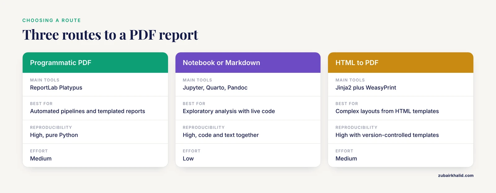
Before writing code, choose a route. Each has trade-offs in effort, flexibility, and reproducibility.
| Route | Tools | Best for | Reproducibility | Effort |
|---|---|---|---|---|
| Programmatic PDF | ReportLab (Platypus) | Fully automated pipelines, templated reports that regenerate on every run | High, pure Python | Medium |
| Notebook or Markdown | Jupyter, Quarto, Pandoc | Exploratory analysis, documents that mix narrative with live code | High, code and text live together | Low |
| HTML to PDF | Jinja2 plus WeasyPrint | Reports with complex layouts, reuse of HTML templates | High with version-controlled templates | Medium |
The programmatic route is what most production pipelines use. ReportLab is the library behind automated PDF generation in a range of published Python systems, from certificate builders [7] to spam-filtering dashboards that emit an automatically created PDF report summarizing detected patterns [8]. The notebook route is grounded in the dynamic documents tradition, where live code, plain text, and rendered output combine into PDF, HTML, or Word formats with minimal effort [9]. The HTML route gives the most layout control and is worth learning once you outflow simple templates.
A fourth option deserves mention. VueGen is a Python package that automates report creation from a directory of bioinformatics outputs, including plots, tables, networks, Markdown text, and HTML components, and emits documents in PDF, HTML, DOCX, and ODT as well as presentations, notebooks, and Streamlit apps [10]. If your goal is to standardize reporting across a lab without writing template code, studying how VueGen structures its report builders is instructive even if you end up writing your own.
The rest of this guide walks through the programmatic route in full, because once you understand it, the other routes become variations on the same analysis-and-figure layer.
Step-by-Step: Generate a Bioinformatics Report in Python (PDF)
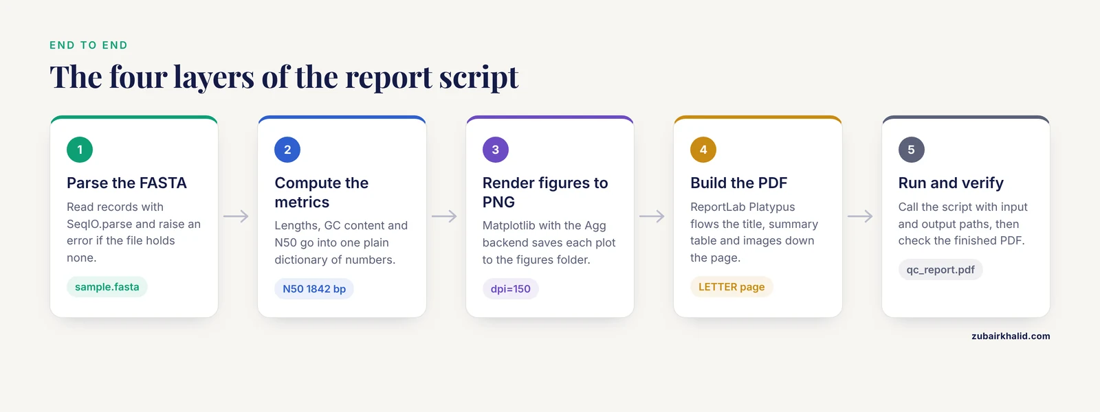
This walkthrough builds a sequence quality-control report from a multi-FASTA file. The same skeleton works for a BLAST hit summary, a variant table, or a differential expression result set. If you are new to Biopython, the official tutorial is the canonical reference, and the Bio.SeqIO module used below is the standard interface for reading sequence files.
Step 1: Set Up the Environment
Create an isolated environment so that package versions stay pinned and reproducible.
conda create -n reportenv python=3.11
conda activate reportenv
pip install biopython pandas matplotlib reportlab
If you use pip without conda, the same four packages install with the single command above. Verify the installation:
python -c "import Bio, matplotlib, reportlab, pandas; print(Bio.__version__)"Expected output is a version string such as 1.83. Any version of Biopython 1.79 or newer supports the gc_fraction function used below.
Write a requirements.txt with the exact versions installed (pip freeze > requirements.txt) and commit it alongside your script. Published pipelines treat version pinning as part of the deliverable, not an afterthought.
Step 2: Parse Sequences and Compute Metrics
FASTA is the plain-text format for nucleotide and protein sequences, where each record starts with a > header line followed by the sequence. GC content is the percentage of bases that are guanine or adenine pairing partners guanine and cytosine, calculated as (G + C) divided by total bases times 100. N50 is the length of the sequence at which half of all bases in the dataset sit in sequences of that length or longer, a standard summary statistic for assembly quality.
Create a file called make_report.py and add the analysis layer:
from pathlib import Path
from Bio import SeqIO
from Bio.SeqUtils import gc_fraction

def parse_fasta(path):
    records = list(SeqIO.parse(path, "fasta"))
    if not records:
        raise ValueError(f"No sequences found in {path}")
    return records

def summarize(records):
    lengths = [len(r.seq) for r in records]
    gc_values = [gc_fraction(r.seq) * 100 for r in records]
    sorted_lengths = sorted(lengths, reverse=True)
    half_total = sum(lengths) / 2
    running = 0
    n50 = 0
    for value in sorted_lengths:
        running += value
        if running >= half_total:
            n50 = value
            break
    return {
        "count": len(records),
        "min": min(lengths),
        "max": max(lengths),
        "mean": sum(lengths) / len(records),
        "n50": n50,
        "mean_gc": sum(gc_values) / len(gc_values),
        "lengths": lengths,
        "gc_values": gc_values,
    }

records = parse_fasta("sample.fasta")
stats = summarize(records)
print(f"Parsed {stats['count']} sequences")
print(f"Mean GC: {stats['mean_gc']:.1f}%")
print(f"N50: {stats['n50']} bp")
For a test file with 24 sequences, expected console output looks like this:
Parsed 24 sequences
Mean GC: 51.3%
N50: 1842 bp
The exact numbers depend on your input. The point of printing them is that you confirm the analysis layer works before any PDF code runs. Debugging two layers at once is the most common way beginners lose an afternoon.
Step 3: Generate Figures with Matplotlib
Figures must be written to disk as PNG files before ReportLab can embed them. Force the non-interactive Agg backend so the script also runs on headless servers and in scheduled jobs.
import matplotlib
matplotlib.use("Agg")
import matplotlib.pyplot as plt

PNG_DIR = Path("figures")
PNG_DIR.mkdir(exist_ok=True)

def plot_length_histogram(lengths, out_path):
    fig, ax = plt.subplots(figsize=(6, 4), dpi=150)
    ax.hist(lengths, bins=20, color="#2c7fb8", edgecolor="white")
    ax.set_xlabel("Sequence length (bp)")
    ax.set_ylabel("Number of sequences")
    ax.set_title("Sequence length distribution")
    fig.tight_layout()
    fig.savefig(out_path)
    plt.close(fig)

def plot_gc_scatter(lengths, gc_values, out_path):
    fig, ax = plt.subplots(figsize=(6, 4), dpi=150)
    ax.scatter(lengths, gc_values, s=24, alpha=0.7, color="#d95f0e")
    ax.set_xlabel("Sequence length (bp)")
    ax.set_ylabel("GC content (%)")
    ax.set_title("GC content vs sequence length")
    fig.tight_layout()
    fig.savefig(out_path)
    plt.close(fig)
Three parameters matter here:
dpi=150controls raster resolution. At 150 dpi, a 6 by 4 inch figure is 900 by 600 pixels, which is crisp in a PDF without inflating file size. Raising it to 300 doubles both dimensions and file size.figsizesets the aspect ratio. Keep it consistent with the width and height you pass to the ReportLabImageflowable, or your figures will be silently stretched.plt.close(fig)releases memory. In a loop that renders dozens of figures, omitting this line is a reliable way to exhaust RAM.
The pattern of computing values and rendering them as diagrams for automatic inclusion in a PDF report generalizes far beyond sequence analysis. The same architecture underpins automated engineering tools that calculate results and emit a PDF report containing calculations, reaction forces, and graphical diagrams built with Matplotlib [11].
Step 4: Build the PDF with ReportLab
ReportLab's Platypus layer (Page Layout and Typography Using Scripts) treats a document as a list of flowables: paragraphs, tables, images, and spacers that flow down the page and break automatically. Build the report layer like this:
from reportlab.lib import colors
from reportlab.lib.pagesizes import LETTER
from reportlab.lib.styles import getSampleStyleSheet
from reportlab.lib.units import inch
from reportlab.platypus import (
    Image, PageBreak, Paragraph, SimpleDocTemplate, Spacer, Table, TableStyle,
)

def build_pdf(stats, records, pdf_path):
    styles = getSampleStyleSheet()
    story = []

    story.append(Paragraph("Sequence QC Report", styles["Title"]))
    story.append(Paragraph(
        "Generated with Python, Biopython, Matplotlib, and ReportLab",
        styles["Normal"],
    ))
    story.append(Spacer(1, 12))

    rows = [
        ["Metric", "Value"],
        ["Sequence count", str(stats["count"])],
        ["Shortest sequence (bp)", str(stats["min"])],
        ["Longest sequence (bp)", str(stats["max"])],
        ["Mean length (bp)", f"{stats['mean']:.0f}"],
        ["N50 (bp)", str(stats["n50"])],
        ["Mean GC content", f"{stats['mean_gc']:.1f}%"],
    ]
    table = Table(rows, colWidths=[2.5 * inch, 2.5 * inch])
    table.setStyle(TableStyle([
        ("BACKGROUND", (0, 0), (-1, 0), colors.HexColor("#2c7fb8")),
        ("TEXTCOLOR", (0, 0), (-1, 0), colors.white),
        ("FONTNAME", (0, 0), (-1, 0), "Helvetica-Bold"),
        ("GRID", (0, 0), (-1, -1), 0.5, colors.grey),
        ("VALIGN", (0, 0), (-1, -1), "MIDDLE"),
        ("TOPPADDING", (0, 0), (-1, -1), 4),
        ("BOTTOMPADDING", (0, 0), (-1, -1), 4),
    ]))
    story.append(table)
    story.append(Spacer(1, 16))

    story.append(Paragraph("Length Distribution", styles["Heading2"]))
    story.append(Image(str(PNG_DIR / "length_hist.png"),
                       width=5.5 * inch, height=3.67 * inch))
    story.append(PageBreak())

    story.append(Paragraph("GC Content vs Length", styles["Heading2"]))
    story.append(Image(str(PNG_DIR / "gc_scatter.png"),
                       width=5.5 * inch, height=3.67 * inch))

    doc = SimpleDocTemplate(
        str(pdf_path),
        pagesize=LETTER,
        title="Sequence QC Report",
        author="Automated QC pipeline",
    )
    doc.build(story)
Key parameters:
pagesize=LETTERsets an 8.5 by 11 inch page. UseA4for European collaborators. Page size changes the usable width, so figure widths should be reviewed if you switch.colWidthsin theTableconstructor fixes column widths in points or inches. Without it, ReportLab distributes width by content, which produces cramped tables when one cell contains a long string.titleandauthorwrite PDF document metadata, which is what appears in the browser tab and in reference managers.- The
Imagewidth and height pair must match the source aspect ratio (6 by 4 inches gives a 1.5 ratio, so 5.5 wide means 3.67 tall) to avoid distortion.
Step 5: Assemble and Run the Full Script
Wire the layers together behind a command-line interface so the script is reusable:
import sys

def main():
    if len(sys.argv) != 3:
        sys.exit("Usage: python make_report.py <input.fasta> <output.pdf>")
    fasta_path = Path(sys.argv[1])
    pdf_path = Path(sys.argv[2])

    records = parse_fasta(fasta_path)
    stats = summarize(records)

    plot_length_histogram(stats["lengths"], PNG_DIR / "length_hist.png")
    plot_gc_scatter(stats["lengths"], stats["gc_values"], PNG_DIR / "gc_scatter.png")

    build_pdf(stats, records, pdf_path)
    print(f"Parsed {stats['count']} sequences")
    print(f"N50: {stats['n50']} bp")
    print(f"Mean GC: {stats['mean_gc']:.1f}%")
    print(f"Report written to {pdf_path}")

if __name__ == "__main__":
    main()
Run it:
python make_report.py sample.fasta qc_report.pdfExpected output:
Parsed 24 sequences
N50: 1842 bp
Mean GC: 51.3%
Report written to qc_report.pdf
The finished PDF has three pages: a title and summary table, the length histogram, and the GC scatter plot. Re-running the script after changing the input regenerates every number and figure, which is the property that makes automated reporting valuable compared with hand-assembled documents [3].
Step 6: Verify the Output Is Correct
Open the PDF and check four things:
- Cross-check one metric by hand. Compute GC content of the shortest sequence with an independent tool or a one-liner such as
python -c "from Bio.SeqUtils import gc_fraction; from Bio import SeqIO; print(gc_fraction(next(SeqIO.parse('sample.fasta','fasta')).seq) * 100)"and compare it with a spot calculation. - Confirm figures are not stretched. The circles in the scatter plot should be round, not ellipses. Ellipse shapes mean the width and height passed to
Imagedo not match the figure aspect ratio. - Confirm page breaks land between sections, not in the middle of a table. If a table splits awkwardly, insert a
SpacerorPageBreakbefore it, or wrap the table in aKeepTogetherflowable. - Check file size. A report with two 150 dpi PNGs should be well under 2 MB. A 50 MB PDF usually means a figure was saved at an extreme dpi or a vector figure embedded a huge dataset.
For automated verification, add a smoke test that builds the report from a tiny fixture FASTA and asserts the PDF exists and is larger than some minimum size:
def test_report_builds(tmp_path):
    pdf_path = tmp_path / "test_report.pdf"
    records = parse_fasta("tests/fixtures/tiny.fasta")
    stats = summarize(records)
    build_pdf(stats, records, pdf_path)
    assert pdf_path.exists() and pdf_path.stat().st_size > 10000
Run it with pytest. This catches the most common silent failure mode, where a refactor of the plotting code breaks the report months later and nobody notices until a collaborator opens the PDF.
Alternative: Notebook and Markdown-Based Reports
If your report is narrative-heavy, with interpretation paragraphs interleaved with code and figures, a notebook is often faster than Platypus. The dynamic documents approach combines live code, plain text, and expressions to generate PDF, HTML, or Word output including the numerical and graphical results, with the code itself properly formatted, at minimal effort [9]. The practical workflow is:
- Write the analysis in a Jupyter notebook with Markdown cells between code cells.
- Export with
jupyter nbconvert, to pdf report.ipynb, which requires a LaTeX toolchain, or convert to HTML and print to PDF from the browser, which does not. - Commit the notebook so the executed output and the code travel together.
Pandoc offers a similar path from a Markdown file: pandoc report.md -o report.pdf converts Markdown with embedded figure references into a typeset PDF. This route needs the Pandoc binary plus a LaTeX engine installed on the system, which is the main friction point on machines you do not control.
Choose the notebook route when the report doubles as the analysis record. Choose ReportLab when the report is a standardized deliverable regenerated on a schedule or inside a pipeline. Production pipelines often do both: the engine emits an HTML report with dynamic visualization for interactive exploration [2] and a static PDF for archiving and sharing. VueGen formalizes exactly this, accepting a directory of outputs and producing PDF, HTML, DOCX, and presentation formats from the same source files [10].
Common Errors and Fixes
ModuleNotFoundError: No module named 'Bio'
Biopython is not installed in the interpreter you are running. Run pip install biopython inside the same environment that Python resolves, and verify with which python on macOS and Linux or where python on Windows. This error almost always means the terminal is using a different environment than the one where you installed packages.
ModuleNotFoundError: No module named 'reportlab'
Same cause as above, different package. If you installed with pip install reportlab but run the script from an IDE, confirm the IDE's interpreter matches the environment. In VS Code, check the interpreter selector in the status bar.
FileNotFoundError: [Errno 2] No such file or directory: 'sample.fasta'
The path is relative to the working directory, not the script location. Run pwd to see where you are, or convert paths to absolute with Path("sample.fasta").resolve() and print the result while debugging.
ValueError: No sequences found in sample.fasta
The parser found the file but no records. Check that the file starts with a > header line and uses standard FASTA formatting. A file exported with Windows line endings usually still parses, but a file with a stray blank first line or a trailing format tag will not.
Black squares or encoding errors for Greek letters and other symbols
ReportLab's built-in fonts (Helvetica, Times-Roman, Courier) cover Latin-1 characters only. Units such as µ and symbols such as α either raise an encoding error or render incorrectly depending on the ReportLab version. Register a TrueType font that covers your characters with pdfmetrics.registerFont(TTFont("DejaVu", "DejaVuSans.ttf")) and set the style's font name accordingly, or replace the characters with ASCII equivalents such as "uM" for micromolar.
ReportLab refuses a Paragraph containing raw "&", "<", or ">"
The Paragraph flowable parses a subset of XML, so an unescaped ampersand raises a parse error with a message pointing at the offending text. Escape these characters or pass text through xml.sax.saxutils.escape() before wrapping it in a Paragraph.
Figures appear cropped or have clipped labels
You saved without fig.tight_layout() or embedded the PNG with dimensions that do not match the aspect ratio. Add fig.tight_layout() before savefig, and compute the embed height as width divided by the figure's width-to-height ratio.
pandoc: command not found
The Markdown route requires the Pandoc executable, which is separate from any Python package. Install it with conda install -c conda-forge pandoc or from the project website, then retry the conversion. The same applies to the LaTeX engine that Pandoc needs for direct PDF output.
Common Mistakes and Limitations
- Mixing analysis and reporting code. If metric computation lives inside the PDF builder, you cannot test the analysis or regenerate the report without rerunning the analysis. Keep the layers separate, as the walkthrough does, and pass a plain data dictionary between them.
- Not recording provenance in the report itself. Every report should state the input filenames, their checksums, the script version, and package versions. Pipelines that validate reproducibility treat this metadata as part of the deliverable, not decoration [3]. A reader who cannot tell which run produced the PDF has a decorative document.
- Treating the report as the analysis. A handsome PDF full of plots is not a quality assessment unless the plots have interpretation attached. MSPypeline succeeds because its QC figures and statistical inference plots feed standardized interpretive steps, not because it draws charts [4]. Decide in advance which values are passing and which trigger a warning, and encode that rule in the script so the narrative text is generated from the data, the way the dynamic rule-based interpretation engine in the public health pipeline generates its textual conclusions from statistical results [3].
- Choosing the output format for the wrong audience. A static PDF cannot zoom into a cluster of points or filter a table. When reviewers need interactivity, emit HTML alongside the PDF, as pipelines that pair static outputs with dynamic visualization reports already do [2]. When the audience includes people who edit text, DOCX is friendlier than PDF [10].
- Unpinned dependencies. A report script that works today can break after a Matplotlib major release changes default styling or a Biopython release renames a function. Pin versions in
requirements.txtand test after upgrades. - Assuming figures transfer at print quality. A PNG at 72 dpi looks fine on screen and unacceptable on paper. Pick 150 dpi as a floor for reports that will be printed, and 300 dpi for anything approaching publication.
- Forgetting the PDF is a snapshot. The document reflects the input file at the moment the script ran. If the upstream data changes, the PDF does not. Schedule regeneration or re-run manually after data updates, and date-stamp the title page so stale reports are obvious.
A final limitation is scope. The script presented here computes descriptive statistics only. Real quality control decisions, such as whether an assembly is good enough to proceed, depend on the sequencing platform, sample type, and experimental goals, and require domain judgment that no report template supplies.
Frequently Asked Questions
Can I generate a bioinformatics report in Python as a PDF without writing HTML or CSS?
Yes. The ReportLab route in this guide produces a complete PDF using only Python objects such as Paragraph, Table, and Image, with no markup languages involved. HTML-based routes are optional, not required.
Which library is best, ReportLab or WeasyPrint?
Use ReportLab when you want a pure-Python dependency and programmatic layout control, and WeasyPrint when you already have or want HTML and CSS templates. ReportLab is the library used across a wide range of published automated PDF systems [7][8], while WeasyPrint excels at converting rich HTML layouts.
How do I put Matplotlib plots into the PDF?
Save each figure with fig.savefig(path) and embed the PNG file with the ReportLab Image flowable, matching the width and height to the figure's aspect ratio. Do not try to pass a Matplotlib figure object directly to ReportLab.
Can the report regenerate automatically on a schedule?
Yes. Because the script takes input and output paths as arguments, you can run it from cron, a CI job, or a pipeline manager on any schedule. Keeping the analysis, plotting, and PDF layers as separate functions makes the scheduled run identical to your interactive run.
Does this work with Biopython objects like SeqRecord directly?
The analysis layer reads SeqRecord objects through SeqIO.parse, but the report layer receives plain Python numbers and strings. Keeping it that way makes the report builder reusable for inputs from any source, not just FASTA files.
What if my report needs dozens of figures and gets slow?
Render figures once to PNG files, close each figure with plt.close(fig) to free memory, and reuse the PNGs if the report is rebuilt. For very large documents, build the story in sections and write a chapter per page.
Can I produce HTML or DOCX versions of the same report?
Yes. If you structure the report content as a list of neutral items (headings, paragraphs, tables, image paths), you can render that list through ReportLab for PDF, python-docx for DOCX, or a Jinja2 template for HTML. The public health pipeline in the literature takes the python-docx path for Word output [3], and VueGen demonstrates the multi-format approach at scale [10].
How do I make reruns produce an identical report?
Pin package versions, avoid timestamps or random seeds in the content, and record input file checksums so you can prove the inputs did not change. If the report includes a generation timestamp, place it in a fixed footer position and accept that the PDF bytes will differ while the content stays identical.
Sources
- Bioinformatics calls the school: Use of smartphones to introduce Python for bioinformatics in high schools
- Abstract 4956: A fast and efficient bioinformatics analysis workflow for processing reads from single-cell multiomics assays captured on a microwell-based platform
- A Reproducible Python-Based Computational Pipeline for Real-Time Ingestion, Advanced Analysis, and Dynamic Reporting of Public Health Data: A Systems Validation Study
- MSPypeline: a python package for streamlined data analysis of mass spectrometry-based proteomics
- multiPhATE: bioinformatics pipeline for functional annotation of phage isolates
- Biofoundry-Scale DNA Assembly Validation Using Cost-Effective High-Throughput Long-Read Sequencing
- Implementation and Research Report on FormGenie: AI-Based Multi-Language Smart form Automation System
- Intelligent spam filtering and analysis using web automation, report lab, and ensemble machine learning techniques
- Creating Dynamic Documents with R and Python as a Computational and Visualization Tool for Teaching Differential Equations
- VueGen: automating the generation of scientific reports
- Development of a Python-Based Tool for Automated Shear Force and Bending Moment Diagram Generation in Structural Analysis