How to Plot Heatmaps for Gene Expression Data in Python

By Dr. Zubair Khalid, DVM, MS, PhD · 2026-11-11

By the end of this article you will be able to take a gene-by-sample expression matrix, scale it correctly, draw a static heatmap with seaborn.heatmap, build a hierarchically clustered version with sns.clustermap, attach colored annotation bars for your experimental groups, save a publication-quality file, and debug the errors that most commonly break this workflow. Everything runs on a standard laptop with Python 3.9 or newer, pandas, numpy, matplotlib, seaborn, and scipy.

A heatmap is a rectangular grid in which each cell's color encodes a numeric value. For gene expression, rows are genes, columns are samples, and color encodes abundance. Done well, a heatmap shows co-expression blocks, condition-specific signatures, and outlier samples in a single glance. Done badly, it shows the arbitrary choices you made in the plotting code. This guide is written so you make the right choices on purpose.

Python for Bioinformatics: Where Heatmaps Fit

Python has become a default implementation language for bioinformatics tooling. Recent releases in the field cover elemental imaging visualization [1], evaluation and plotting utilities for designed biological sequences [2], scalable phylogenomic visualization [3], Sort-seq variant scoring that ships with built-in heatmap visualizations [4], and flexible similarity matrix construction for omics clustering [5]. Visualization libraries such as seaborn sit underneath this ecosystem as the shared rendering layer, which means learning seaborn.heatmap and seaborn.clustermap pays off across many of these tools.

Heatmaps also connect to larger analysis workflows. Spatial transcriptomics protocols emphasize script-based execution with explicit parameter rationales so results are reproducible [6]. Pipelines for small RNA sequencing are distributed as containerized Nextflow workflows with companion visualization apps [7]. R and Python ecosystems increasingly interoperate, and R/Bioconductor infrastructure such as Spectra is explicitly designed to integrate with third-party Python tools [8]. End-to-end frameworks like the Spatial Omics Toolkit are implemented in both R and Python on vendor-neutral formats [9]. Your heatmap code should be written as a script or notebook that a colleague can rerun, not as a one-off session, and this guide follows that convention.

One caution before the code. Visual inspection of high-dimensional data is prone to confirmation bias, and the single-cell field has moved toward principled statistical tests precisely because eyeballing two-dimensional summaries can mislead [10]. Treat the heatmap as a hypothesis generator, not as evidence.

Step 0: Install the Environment

Create an isolated environment so library versions are pinned and reproducible:

python -m venv heatmap-env
source heatmap-env/bin/activate
pip install pandas numpy matplotlib seaborn scipy

On Windows use heatmap-env\Scripts\activate instead of the source line. Check the install:

python -c "import seaborn as sns; print(sns.__version__)"

You should see 0.13.x or similar. Scipy is optional for sns.heatmap but mandatory for sns.clustermap, which delegates dendrogram construction to scipy.cluster.hierarchy. For an even more reproducible setup, write the package list to a file and install from it:

pip freeze > requirements.txt
pip install -r requirements.txt

Step 1: Get Your Matrix Into the Right Shape

Seaborn expects a single pandas DataFrame where every cell is numeric. For a gene expression heatmap the convention is genes as rows and samples as columns. Load a count matrix or a normalized table from CSV:

import pandas as pd

expr = pd.read_csv("counts.tsv", sep="\t", index_col=0)
print(expr.shape)        # (rows, columns), e.g. (20000, 12)
print(expr.dtypes.value_counts())

The index_col=0 argument uses the first column (gene IDs) as row labels. Confirm three things before plotting:

1. Every column is numeric. If your file came from Excel, missing values are often the string "NA" or "-", which forces the whole column to object dtype.
2. Row labels are unique. Duplicated gene symbols break clustermap.
3. Missing values are true NaN, not sentinel numbers such as 0 or -999. A zero in RNA-seq counts is a real observation, but a zero in a log-space matrix usually means "not measured."

Fix the common cases like this:

expr = expr.apply(pd.to_numeric, errors="coerce")   # strings become NaN
expr = expr.loc[~expr.index.duplicated(keep="first")]
expr = expr.dropna(axis=0, how="any")               # or impute instead

Dropping genes with any missing value is acceptable for a focused panel of a few hundred genes. For a genome-wide matrix, dropping can silently remove thousands of genes, so count what you lose with expr.shape before and after.

Step 2: Choose a Scale Before You Choose a Color

The single biggest determinant of what a heatmap tells you is the scale of the numbers, not the colormap. Raw counts are dominated by gene length and library size, so genes with high baseline expression saturate the color scale and everything else fades to the bottom of the range. Normalize first, then transform, then optionally standardize.

The three standard choices:

• CPM or TPM (counts or transcripts per million) puts genes on a comparable abundance scale. Good when absolute abundance matters.
• log2(TPM + 1) or log2(counts per million + 1) compresses the dynamic range so a heatmap is not dominated by three hyper-expressed genes. This is the default choice for most expression heatmaps.
• Per-gene z-score computes, for each gene, (value - mean across samples) / SD across samples. Every row then has mean 0 and SD 1, so color encodes relative change within a gene rather than absolute abundance. Use this when the question is "which genes go up in which samples," which is the question most heatmaps are actually asking.

The explicit pandas computation, which is transparent and version-proof:

z = expr.sub(expr.mean(axis=1), axis=0).div(expr.std(axis=1), axis=0)

expr.mean(axis=1) computes one mean per row. Subtracting it with axis=0 alignment subtracts each gene's own mean from that gene's values. Seaborn also offers a built-in z_score and standard_scale argument that performs standardization inside the plotting call, which is a convenient shortcut to the same operation.

Seaborn is flexible about data structures, and recent bioinformatics tools exploit that, from elemental imaging matrices decomposed into single-element data frames [1] to omics similarity matrices evaluated across clustering strategies [5]. Whatever upstream tool produced your matrix, the plotting contract is the same: one numeric DataFrame.

Step-by-Step: Gene Expression Heatmap in Python with Seaborn

Work through this sequence with a small hand-built matrix first so every value is verifiable, then scale up to your real data.

1. Build or load the matrix

import pandas as pd

expr = pd.DataFrame(
    {
        "CTRL_1": [10.2, 3.1, 8.4, 5.5],
        "CTRL_2": [ 9.8, 2.9, 8.1, 5.9],
        "CTRL_3": [10.5, 3.3, 8.6, 5.2],
        "TREAT_1": [12.9, 6.8, 4.2, 5.7],
        "TREAT_2": [13.1, 7.2, 4.0, 5.4],
        "TREAT_3": [12.6, 6.5, 4.5, 5.8],
    },
    index=["GENE1", "GENE2", "GENE3", "GENE4"],
)
print(expr.round(1))

Printed output:

        CTRL_1  CTRL_2  CTRL_3  TREAT_1  TREAT_2  TREAT_3
GENE1     10.2     9.8    10.5     12.9     13.1     12.6
GENE2      3.1     2.9     3.3      6.8      7.2      6.5
GENE3      8.4     8.1     8.6      4.2      4.0      4.5
GENE4      5.5     5.9     5.2      5.7      5.4      5.8

Read the biology from the table first. GENE1 goes up with treatment, GENE2 goes up strongly, GENE3 goes down, GENE4 does nothing. Your heatmap must reproduce those four statements in color.

2. Z-score each gene

z = expr.sub(expr.mean(axis=1), axis=0).div(expr.std(axis=1), axis=0)
print(z.round(2))

Printed output:

        CTRL_1  CTRL_2  CTRL_3  TREAT_1  TREAT_2  TREAT_3
GENE1   -0.66   -0.98   -0.35     0.75     0.90     0.33
GENE2   -1.04   -1.14   -0.94     0.95     1.15     1.01
GENE3    0.99    0.68    1.09    -0.96    -1.06    -0.74
GENE4   -0.47    1.40   -1.40     0.47    -0.94     0.94

Each row now averages to 0. Check it: z.mean(axis=1) returns values at the level of floating-point noise, roughly 1e-16 or smaller. If it does not, your subtraction was misaligned.

3. Draw the heatmap

import seaborn as sns
import matplotlib.pyplot as plt

fig, ax = plt.subplots(figsize=(5.5, 4))
sns.heatmap(
    z,
    cmap="vlag",
    center=0,
    vmin=-1.2, vmax=1.2,
    linewidths=0.5,
    linecolor="white",
    cbar_kws={"label": "Row z-score"},
    ax=ax,
)
ax.set_ylabel("")
ax.set_xlabel("")
fig.tight_layout()
fig.savefig("expression_heatmap.png", dpi=300, bbox_inches="tight")
fig.savefig("expression_heatmap.pdf", bbox_inches="tight")

Expected result: a 4-by-6 grid on a diverging red-to-blue palette (vlag runs blue for negative, red for positive), symmetric around zero. GENE1 and GENE2 show a blue-to-red left-to-right transition, GENE3 the reverse, GENE4 shows weak mixed colors near the pale center of the scale. The colorbar runs from -1.2 to 1.2 with the label "Row z-score." GENE4's near-zero z-scores rendering as washed-out pale cells is the correct behavior, not a bug.

4. Verify the figure against the data

Three checks that catch most plotting errors:

# Check 1: row means are zero
assert z.mean(axis=1).abs().max() < 1e-10

# Check 2: the displayed range matches what you asked for
print(z.values.min(), z.values.max())   # compare against vmin, vmax

# Check 3: spot-check one cell against the raw data
print(z.loc["GENE2", "TREAT_2"])        # should match the printed table above

If the figure disagrees with any of these, fix the data pipeline before touching the plotting code. This habit mirrors the explicit parameter rationales and troubleshooting checkpoints recommended in published spatial transcriptomics workflows [6].

Choosing Colormaps and Limits: A Reference Table

The parameters below control almost everything that matters in sns.heatmap and sns.clustermap.

One colormap rule dominates all others: never use rainbow-style palettes such as "jet" for expression data. Diverging palettes with a meaningful center make sign and magnitude readable simultaneously. Sequential palettes such as "mako" are correct when the data has a natural zero point at the bottom, for example TPM abundance.

Step 5: Cluster Rows and Columns with sns.clustermap

A clustered heatmap reorders rows and columns by hierarchical clustering and draws the dendrograms, which is a tree diagram showing how genes or samples merge into groups at increasing distances. This is where co-expression structure becomes visible. The clustering literature in omics is candid that the choice of similarity measure and clustering strategy materially changes the resulting groups [5], so record your method and metric in the figure caption.

Extend the tutorial data with a second step. First simulate a larger matrix so clustering has something to find:

import numpy as np

rng = np.random.default_rng(0)
n_genes, n_samples = 60, 6
base = rng.normal(8, 1.2, size=(n_genes, 1))
design = np.array([0, 0, 0, 2.5, 2.5, 2.5])
signal = rng.normal(0, 0.3, size=(n_genes, 1)) * design
counts = rng.poisson(np.exp(base + signal))
log_expr = pd.DataFrame(
    np.log2(counts + 1),
    index=[f"G{i:03d}" for i in range(n_genes)],
    columns=["C1", "C2", "C3", "T1", "T2", "T3"],
)
z = log_expr.sub(log_expr.mean(axis=1), axis=0).div(log_expr.std(axis=1), axis=0)

Then cluster:

g = sns.clustermap(
    z,
    cmap="vlag",
    center=0,
    vmin=-2, vmax=2,
    method="average",
    metric="euclidean",
    figsize=(6, 8),
    dendrogram_ratio=0.15,
    cbar_pos=(0.02, 0.82, 0.03, 0.15),
)
g.ax_heatmap.set_xlabel("")
g.ax_heatmap.set_ylabel("")
g.savefig("clustered_heatmap.png", dpi=300, bbox_inches="tight")

Expected result: the three control columns sit adjacent to each other, the three treatment columns sit adjacent to each other, genes with treatment-induced changes form visible red or blue row blocks, and a dendrogram above the columns shows the treatment group joining the control group at the top merge. Genes that vary randomly stay near their original neighbors with pale colors.

Retrieve the reordering that clustering chose, because you will need it to report gene order or to join the figure with other panels:

row_order = g.dendrogram_row.reordered_ind
print(g.data2d.iloc[row_order, :].index[:10].tolist())

g.data2d is the exact matrix seaborn plotted, in final clustered order. Saving it with to_csv() makes the figure fully reproducible.

Step 6: Add Annotation Bars for Groups and Metadata

Annotation bars are thin colored strips alongside the heatmap that mark which samples belong to which condition, batch, or time point. They turn a heatmap from a data summary into an interpretable figure.

condition = pd.Series(
    ["#4c72b0", "#4c72b0", "#4c72b0", "#dd8452", "#dd8452", "#dd8452"],
    index=log_expr.columns,
    name="Condition",
)

g = sns.clustermap(
    z,
    cmap="vlag",
    center=0,
    vmin=-2, vmax=2,
    col_colors=condition,
    figsize=(6, 8),
)
g.savefig("annotated_clustermap.png", dpi=300, bbox_inches="tight")

For multiple annotations, pass a DataFrame instead of a Series, one named column per annotation, with rows keyed by sample ID:

annot = pd.DataFrame({
    "Condition": condition,
    "Batch": ["#55a868", "#55a868", "#c44e52", "#55a868", "#c44e52", "#55a868"],
}, index=log_expr.columns)

g = sns.clustermap(z, col_colors=annot, cmap="vlag", center=0)

The Series name (name="Condition") or the DataFrame column names become the small legend text seaborn draws. If your annotation bar colors appear in the wrong order relative to the heatmap columns, your Series index does not match the DataFrame index exactly, which is the most common cause and is covered in the errors section below.

Handling Large Expression Matrices

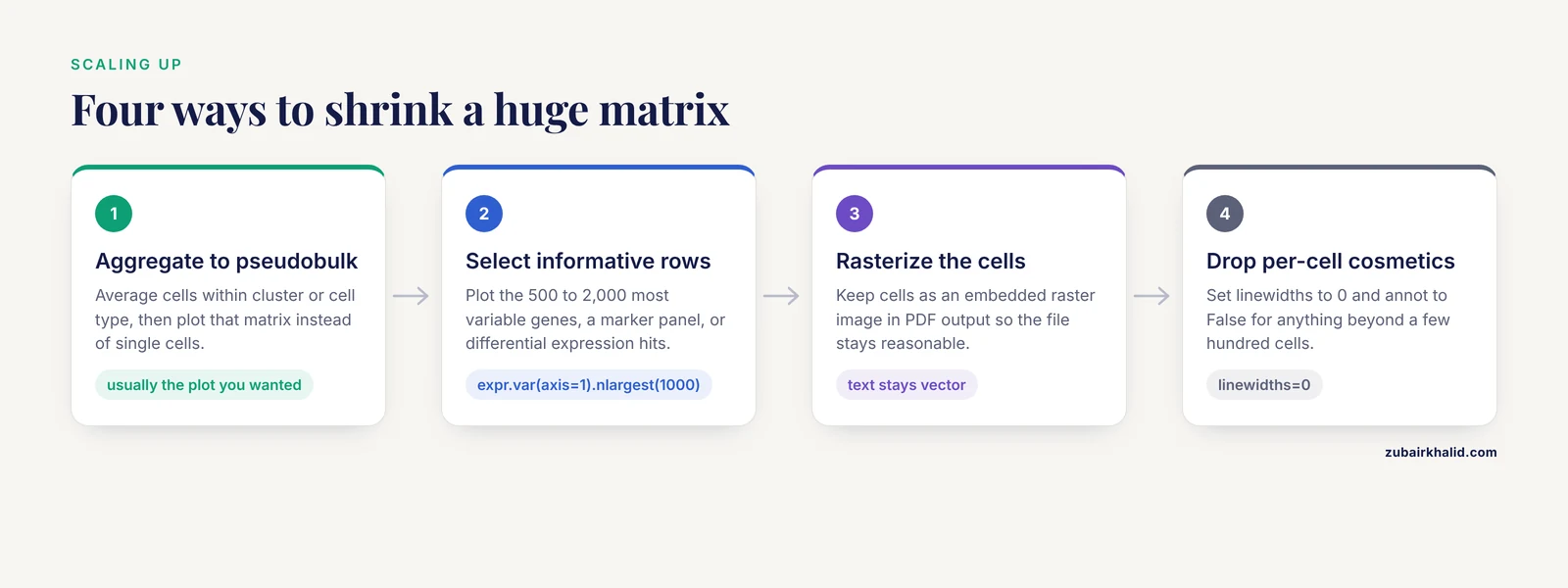
Heatmaps are dense by design, and scale eventually breaks them. A bulk RNA-seq matrix of 20,000 genes by 20 samples plots fine as a clustermap, though rendering 20,000 tiny cells makes the PDF heavy. Single-cell matrices of 20,000 genes by 50,000 cells will not plot at all at cell resolution. The scalable phylogenomics literature describes the same class of problem for large datasets with complex metadata, and solves it by preprocessing and by purpose-built renderers [3]. The highly multiplexed imaging toolbox spatialproteomics demonstrates the practical ceiling by processing images up to gigapixel scale with dedicated pipelines rather than naive plotting calls [11].

Apply the same logic to expression matrices:

1. Aggregate. Average cells within cluster or cell type to get a pseudobulk matrix, then plot that. This is standard practice and usually the plot you wanted anyway.
2. Select informative rows. Plot the 500 to 2,000 most variable genes, a marker gene panel, or differential expression hits. Variability selection with expr.var(axis=1).nlargest(1000).index is one line.
3. Rasterize. For PDF output, keep cells as an embedded raster image so file size stays reasonable while text remains vector. Set rasterized=True on the heatmap artist if your matplotlib version exposes it through g.ax_heatmap children.
4. Turn off per-cell cosmetics. linewidths=0 and annot=False for anything beyond a few hundred cells.

Tips for Publication-Quality Output

These are the adjustments that separate a screen dump from a figure a journal will accept, and they double as a practical checklist of gene expression heatmap python seaborn tips gathered from day-to-day use.

• Fix the color scale across panels. If Figure A shows z-scores from -3 to 3 and Figure B from -1 to 1, readers will compare colors that do not mean the same thing. Pass identical vmin and vmax to every panel.
• Save vector and raster versions. PDF or SVG for the manuscript, PNG at 300 DPI for slides and email. The savefig calls in step 3 do both.
• Label the colorbar. An unlabeled colorbar forces readers to guess whether red means high TPM or high z-score.
• Keep dendrograms honest. If you cluster rows, say so in the caption along with the linkage method and distance metric.
• Sort deliberately when you do not cluster. expr.sort_values(by="TREAT_1", ascending=False) places genes in ranked order, which is often clearer than clustering for small panels.
• Trim dead space. bbox_inches="tight" in savefig removes the margins matplotlib leaves by default.
• Annotate only what fits. Writing numbers in cells works up to roughly 20 by 20. Beyond that, call out specific genes with row labels instead.
• Version your environment. The pipeline literature is emphatic that containerized, fully specified execution is what makes figures reproducible across machines [7], and guided pipelines exist precisely because ad hoc scripting environments are a barrier for many laboratories [12]. A requirements.txt checked into your repository is the minimum.

Common Mistakes and Common Errors

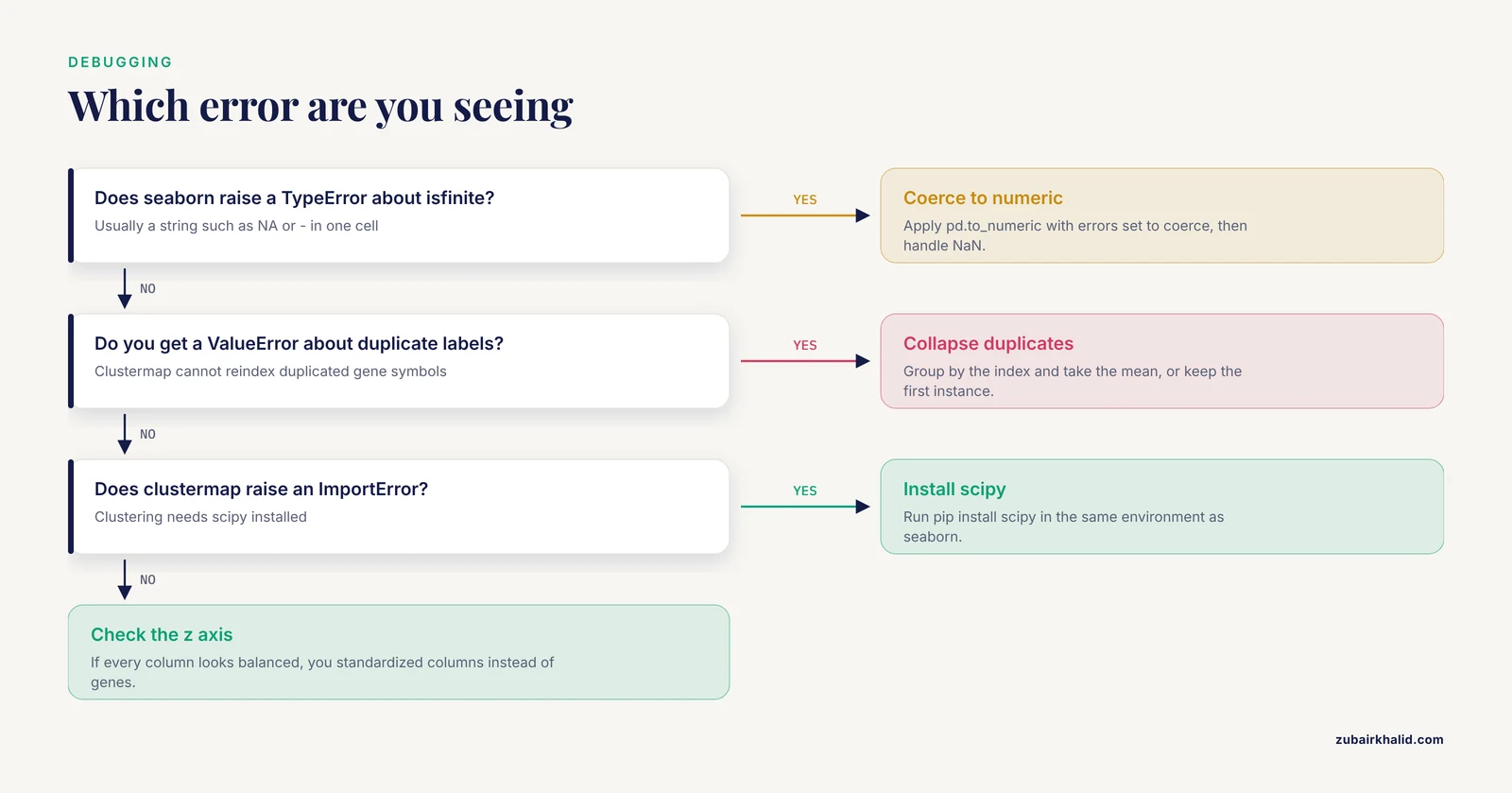
This section pairs the conceptual mistakes behind gene expression heatmap python seaborn common mistakes queries with the exact errors that usually announce them.

Plotting raw counts. Raw counts encode library size and gene length as much as biology. The figure becomes a map of sequencing depth. Normalize to CPM or TPM, log transform, and z-score per gene for relative comparisons.

Z-scoring the wrong axis. Substituting .sub(expr.mean(axis=0), axis=1) standardizes each column instead of each gene. The tell-tale symptom is that every column looks balanced while genes with real changes blend in. Verify with z.mean(axis=1), which must be approximately zero for per-gene z-scores.

Naming your script seaborn.py. Python imports your own file instead of the library and fails with ImportError: cannot import name 'heatmap' from 'seaborn'. Rename the script and delete the pycache folder next to it.

Object dtype leaking in from a spreadsheet. If one cell contains the string "NA", the column becomes object dtype and seaborn raises TypeError: ufunc 'isfinite' not supported for the input types while building the color array. Fix with expr = expr.apply(pd.to_numeric, errors="coerce"), then decide explicitly how to handle the resulting NaN values.

Duplicate gene symbols. Clustermap reorders the index, and duplicated labels raise ValueError: cannot reindex on an axis with duplicate labels or produce silently misaligned annotation colors. Collapse duplicates with expr = expr.groupby(level=0).mean() or keep one instance with expr.loc[~expr.index.duplicated(keep="first")].

Missing scipy for clustermap. Seaborn raises an ImportError stating that the clustering functionality requires scipy. Install it with pip install scipy and rerun.

Unscaled outliers flattening the figure. One gene at 50,000 TPM against a sea of genes near 10 TPM makes everything else one color. Log transform, or set robust=True so color limits come from robust quantiles rather than extremes.

Annotation bars in the wrong order. After clustering, seaborn reorders columns but matches col_colors by index label, not by position. If your colors appear scrambled, print g.data2d.columns and confirm each annotation Series or DataFrame uses those exact labels as its index.

Reading too much into the picture. A clustered heatmap will always show blocks, even under the null hypothesis of no structure, because clustering finds structure in noise by construction. Rigorous single-cell methods were introduced specifically because visual assessment of distributional differences is unstable and open to confirmation bias [10]. Follow up any visually striking block with a statistical test.

Forgetting that z-scores erase magnitude. After per-gene z-scoring, a gene that doubles from 0.1 to 0.2 TPM can look identical to a gene that doubles from 5,000 to 10,000 TPM. Pair z-scored heatmaps with a table of effect sizes, or add a second panel on the log abundance scale.

Checking Your Result End to End

A heatmap is correct when four conditions hold at once. The data in the figure equals the DataFrame you intended, which g.data2d confirms for clustermap and the raw matrix confirms for heatmap. The color limits in the colorbar match your vmin and vmax arguments. The group structure you know independently, for example three controls and three treated samples, appears as adjacent columns in a clustered heatmap, and the annotation bar colors line up with those groups. Finally, spot-check two or three individual cells against the source table. If all four pass, the remaining risk is interpretive, not technical, and belongs in your statistics rather than your plotting code.

Next Steps: Annotations with Biopython and Beyond

A heatmap with gene IDs is more useful with functional annotation. This is where a Biopython tutorial approach earns its place in your toolkit. Biopython's Bio.Entrez module queries the NCBI Entrez system directly from Python:

from Bio import Entrez

Entrez.email = "[email protected]"
gene_ids = ["7157", "7124"]  # NCBI GeneIDs, for example TP53 and TNF
handle = Entrez.esummary(db="gene", id=",".join(gene_ids))
records = Entrez.read(handle)
handle.close()
for rec in records["DocumentSummarySet"]["DocumentSummary"]:
    print(rec["Name"], rec["Description"])

Set a real email address, which NCBI requires so it can contact you about excessive request rates, and add a short delay between calls with time.sleep(0.34) to stay under three requests per second. You can pull gene descriptions, chromosome locations, and summary text this way and write them into row labels or an annotation column. From there, natural next steps are marker gene panels for single-cell data, integration with differential expression results from tools such as DESeq2 exported as CSV, and multi-panel figures where several heatmaps share a color scale. The tools cited throughout this article, from sequence evaluation with visualization diagnostics [2] to cross-ecosystem R and Python integration [8], are reasonable places to see how small plotting scripts like the ones here grow into full analysis frameworks.

Frequently Asked Questions

What is the difference between sns.heatmap and sns.clustermap?

sns.heatmap draws the matrix in the order you give it with no reordering, while sns.clustermap runs hierarchical clustering on rows, columns, or both, reorders the data, and draws dendrograms. Use heatmap when the row or column order is meaningful, use clustermap when you want structure discovery.

Should I plot raw counts, TPM, or z-scores?

Never raw counts, which reflect library size as much as expression. Use log2(TPM + 1) when absolute abundance matters, and per-gene z-scores when the question is relative change across conditions, which is the case for most expression heatmaps.

How do I handle missing values in an expression matrix?

Coerce non-numeric entries to NaN with pd.to_numeric(errors="coerce"), then either drop genes with dropna(axis=0) for small panels or impute for genome-wide matrices, because dropping silently removes many genes when data is sparse.

Why do all the cells in my heatmap look the same color?

Either one or a few extreme values have stretched the color scale so everything else falls in a narrow band, or you forgot to scale data with very different per-gene ranges. Log transform, z-score, or pass explicit vmin and vmax values.

How do I add colored bars showing which samples belong to which group?

Pass a pandas Series (one color per sample, indexed by sample ID) to the col_colors argument of sns.clustermap, or a DataFrame for several annotation bars at once. Match the index labels exactly to the DataFrame column names.

What do I do when my matrix is too large to plot?

Aggregate cells into pseudobulk groups, select the most variable genes or a marker panel to reduce rows, rasterize large cells in vector output, and turn off per-cell annotations and grid lines. Plotting tens of thousands of raw single-cell columns is neither feasible nor informative.

Do I need scipy installed to use clustermap?

Yes. Seaborn delegates dendrogram construction to scipy's clustering functions and raises an ImportError without it, so run pip install scipy in the same environment where seaborn is installed.

How do I recover the gene order that clustermap chose?

Read g.dendrogram_row.reordered_ind for row positions and g.data2d for the fully reordered matrix, then save it with to_csv() so the exact figure content is reproducible from your script.

Sources

1. ScaleBarOn and Muad'Data: simple Python tools for elemental imaging data visualization and comparative scaling.
2. seqme: a Python library for evaluating biological sequence design from generative models.
3. An Integrated Ecosystem for Analysis and Visualization of Large-Scale Phylogenomic Data Combining ETE Toolkit, TreeProfiler, and PhyloCloud for Scalable Phylogenomic Analysis.
4. sortscore: Sort-seq MAVE scoring and visualization using Python.
5. PySimi: a unified framework for similarity measure evaluation in spectral clustering with applications to omics data.
6. A Practical Workflow for Spatial Transcriptomics Data Analysis: From Data Acquisition to Advanced Analyses.
7. PerSeqPIPE: Nextflow workflow for per-sequence analysis of small RNA-sequencing data.
8. An Open Infrastructure for Mass Spectrometry Data in R.
9. A Protocol for Multivariate Data Visualization and Pseudotime Modeling for Analysis of Disease Trajectories Detected by Mass Spectrometry Imaging.
10. Quantifying distribution shifts in single-cell data with scXMatch.
11. Spatialproteomics: an interoperable toolbox for analyzing highly multiplexed fluorescence image data.
12. FetchPA: a guided, end-to-end solution for local ATAC-Seq data processing and analyses.