How to Build a Simple Bioinformatics Pipeline with Galaxy
By Dr. Zubair Khalid, DVM, MS, PhD ·
By the end of this article you will have built and run a complete, reusable analysis pipeline in Galaxy that takes raw RNA-seq FASTQ files through quality control, adapter trimming, alignment to a reference genome, read counting per gene, and a differential expression table with adjusted p values. You will also have converted that point and click analysis into a workflow you can rerun on new samples in minutes, and you will know how to verify each intermediate result instead of trusting a green check mark.
You need three things before you start:
- A web browser. Nothing needs to be installed on your computer.
- A free account on a public Galaxy server such as usegalaxy.org, usegalaxy.eu, or usegalaxy.org.au.
- A small test dataset. If you do not have your own sequencing data, the Galaxy Training Network provides shared test histories with real FASTQ files you can copy into your own history in one click.
Galaxy was designed for exactly this situation. Bioinformatics has a steep learning curve for bench biologists and clinicians, and part of the difficulty is learning to code while also learning the biology and the statistics at the same time. Galaxy separates those two problems. You learn the analytical logic in a graphical interface first, and the code can come later. The Multi-Interface Galaxy Hands-on Training Suite (MIGHTS) project built its entire single-cell training curriculum around this idea, offering parallel button-based and code-based versions of the same analyses so learners can move between the two environments smoothly [1].
What Galaxy Is and Why It Fits a First Pipeline
Galaxy is an open, web-based platform for data-intensive biomedical research. Each server hosts hundreds of bioinformatics tools wrapped behind simple web forms. Every tool you run writes its output into a history, which is a persistent, shareable record of every file and every parameter you used. That history is the backbone of reproducibility. Two years after you run an analysis, you can open the history, see exactly which adapter sequence you trimmed with and which genome build you aligned against, and rerun the whole thing on new data as a workflow.
For a first pipeline, this solves three practical problems:
- No installation. A public Galaxy server runs the tools for you on remote compute, so a laptop with a browser is enough for moderate-sized data.
- Visible provenance. Each dataset in the history remembers the tool, the exact parameter settings, and the input datasets that produced it.
- A gentle path to code. Because the same tools and workflows can be accessed through the interface or through code-based environments, Galaxy has become a recognized gateway into computational biology rather than a dead end that hides how the tools work [1].
A note on scope. This walkthrough builds an RNA-seq differential expression pipeline because it touches every stage a beginner needs to understand: raw read quality, trimming, alignment, counting, and statistics. The same structural approach, upload, QC, process, analyze, wrap into a workflow, applies to whole genome variant calling, metagenomics, proteomics, and single-cell analysis. Published Galaxy workflows such as Model Organism Modifier (MOM), which takes raw short-read whole genome sequencing data and reduces thousands of candidate variants down to a short list for manual curation, follow the identical pattern of ordered steps, tailored filters, and a written tutorial guiding the user through the interface [2].
Before You Start: Accounts, Data, and Conventions
Create an account. Go to usegalaxy.org (or the European or Australian mirror if you are closer to those) and register with an email address. An account is required to keep histories between sessions and to get a meaningful disk quota. Anonymous sessions work for quick tests but the history can be lost.
Understand the interface. Three panels:
- The Tools panel (left) lists every available tool, searchable by name.
- The History panel (right) shows your datasets, colored green (finished successfully), gray (queued or running), or red (failed).
- The Center pane shows the form for whichever tool you clicked, and the output preview for whichever dataset you select.
Set the display and naming conventions now. Rename datasets as you go using the pencil icon. A history full of files named "1: Cutadapt on data 5" becomes unreadable at 12 samples. Use names like wt_rep1_trimmed.fastq. Future you, and anyone you share the history with, will thank you.
Quota reality check. Public servers give registered users a fixed amount of disk space and limit how much you can run at once. For a full-sized mammalian RNA-seq project (12 samples, 30 million paired reads each) you will approach typical quotas, so plan to delete large intermediate files (BAM files can be regenerated) once you no longer need them, or move to a larger allocation. Many institutions host their own Galaxy, and anyone can install their own, but public servers are the right starting point.
Get test data. The cleanest path: open the Galaxy Training Network tutorial for RNA-seq differential expression (training.galaxyproject.org), find its linked example history, and use the history import option under "User → Histories → Import from file" or the "Shared Data → Published Histories" menu. This gives you real FASTQ files plus the reference annotation, so every step below behaves exactly as described. If you have your own reads, upload them with "Upload Data" or from a URL with "Upload File from external web link" (Remote files). After any upload, confirm that Galaxy detected the format as fastqsanger (or fastqsanger.gz for compressed files). Wrong format detection is the single most common source of downstream failures.
Galaxy Bioinformatics Pipeline Tutorial: Step by Step
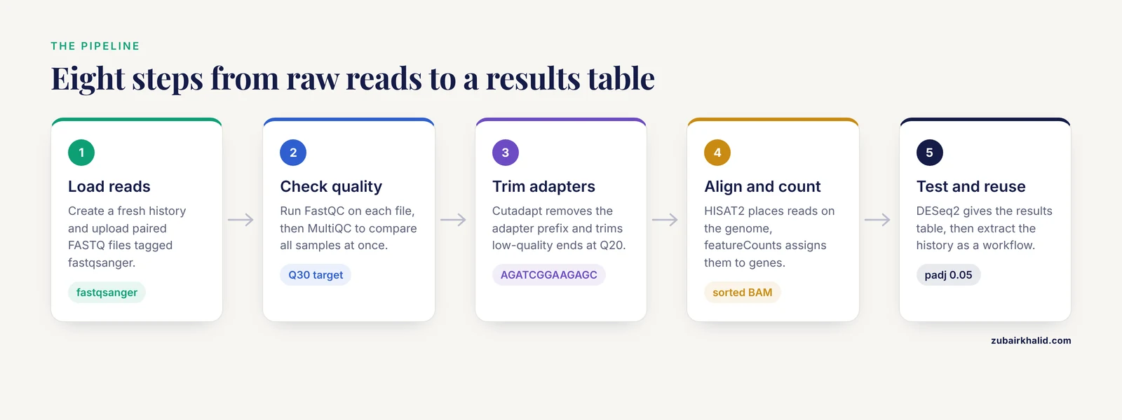
This is the core walkthrough for how to build a simple bioinformatics pipeline with Galaxy. Follow it once with test data end to end, then convert it into a workflow.
A few terms first, since every step depends on them:
- FASTQ is the raw read file format from a sequencer. Each read has a sequence and a per-base quality score encoded as characters.
- Adapters are short synthetic DNA sequences left attached to reads during library preparation. They must be removed before alignment.
- Alignment is the process of placing each read at its position on a reference genome, producing a BAM file (the standard binary alignment format).
- GTF (gene transfer format) is the annotation file that tells the counting tool where genes and exons are on that genome.
- Counts are the number of reads assigned to each gene, the raw input for differential expression statistics.
Step 1: Create a Fresh History and Load Your Reads
- Click the history dropdown (gear icon) and choose Create New History. Rename it, for example,
demo_rnaseq_2026-11. - Open Upload Data. Upload your two paired-end FASTQ files (forward reads R1 and reverse reads R2 for each sample), or paste a URL into the "Paste/Fetch data" tab.
- For each uploaded file, click the pencil icon and check two attributes: the datatype must be
fastqsanger(orfastqsanger.gz) and the database/build must match your organism.
The database/build setting matters more than beginners expect. It tags every dataset with a genome version (for example, mm10 for mouse or GRCh38 for human). Tools that have built-in indexes will use this tag to pick the correct one automatically, and mismatches here are a classic source of silent errors.
Expected history state after this step: two (or more) green datasets, each a few gigabytes at most for test data, showing a read count and a snippet when you click the eye icon. A FASTQ preview looks like four lines per read:
@SRR14863123.1 1 length=75
GATCGGAAGAGCACACGTCTGAACTCCAGTCACATCACGATCTCGTATGC
+SRR14863123.1 1 length=75
FFFFFIIIIIIIIIIIIIIIIIIIIIIIIIIIIIHIIIIIIIIIIIIIH
(Values shown here are illustrative. Your read names and sequences will differ.)
Step 2: Quality Control with FastQC and MultiQC
FastQC computes summary statistics and plots for sequencing data: per-base quality scores, sequence length distribution, GC content, adapter contamination, and sequence duplication.
- Search the tools panel for FastQC (in the "FASTQ Quality Control" section).
- Select your FASTQ files as input. For paired-end data, choose "Collections" or run per-file; FastQC in Galaxy accepts multiple datasets and paired collections.
- Leave the defaults for a first run and click Execute.
Each input produces two outputs: an HTML report and a raw text summary. Open the HTML report with the eye icon. The sections that actually drive decisions are:
- Per base sequence quality. Phred quality scores (a logarithmic scale where Q30 means a 1 in 1,000 chance the base call is wrong). Solid libraries stay above Q30 for most of the read and drop at the very end.
- Adapter Content. If adapter sequence climbs toward the end of reads, you need trimming.
- Overrepresented sequences. Long runs of the same sequence can indicate adapter dimers or contamination.
Run MultiQC next, selecting all the FastQC raw outputs as input. MultiQC aggregates every sample's plots into one HTML report, which is how you spot one bad library out of twelve. Look across the per-base quality plot for samples whose curves sag noticeably below the others.
What "right" looks like: median Phred scores at or above roughly 30 across most read positions, sequence lengths consistent with your expected read length, and adapter content near zero if the library was already trimmed by the sequencing facility.
Step 3: Trim Adapters and Low-Quality Ends with Cutadapt
Cutadapt removes adapter sequences and trims bases below a quality threshold.
- Search for Cutadapt (in "Text Manipulation" on most servers, under NGS tools generally).
- Input: your FASTQ collection or files.
- Key parameters, using Galaxy's form labels:
| Tool | Parameter (Galaxy form label) | What it does | Sensible first value |
|---|---|---|---|
| Cutadapt | Adapter 3' (sequence to trim from the read end) | Removes adapter remnants | AGATCGGAAGAGC (Illumina TruSeq prefix) |
| Cutadapt | Quality filtering | Trims low-quality ends before adapter removal | Q20 |
| Cutadapt | Minimum length | Discards reads shorter than this after trimming | 20 bp |
| HISAT2 | Source / built-in index | Chooses the prebuilt genome index, matched to your dataset's build tag | Your organism build, e.g. mm10 |
| featureCounts | Strandedness | How read orientation maps to gene strands | Match your library protocol, e.g. reverse |
| featureCounts | Gene annotation (GTF) | Defines genes and exons for counting | Same genome build as the alignment index |
| DESeq2 | Design formula | Statistical model, including your comparison factor | ~ condition |
| DESeq2 | FDR / adjusted p value threshold | Controls the false discovery rate in the results table | 0.05 |
- Set the adapter sequence for your library chemistry. The TruSeq adapter prefix
AGATCGGAAGAGCcovers most standard Illumina RNA-seq libraries, but check your library preparation sheet. Using the wrong adapter means Cutadapt finds nothing to remove, which you will detect as unchanged adapter content in the post-trim FastQC report. - Execute, then re-run FastQC on the trimmed output and confirm the Adapter Content plot is now flat.
Expected output: Cutadapt prints a trimming report as its stdout. In Galaxy this appears in the tool's info or a report dataset, looking like:
Total reads processed:        1,204,866
Reads with adapters:            486,103  (40.3%)
Reads written (passing filters): 1,198,912  (99.5%)
Total basepairs processed:   90,364,950
Quality-trimmed:               1,204,177  ( 1.3%)
Total written (filtered):    89,331,220  (98.9%)
(These numbers are illustrative. Your percentages depend on library quality.) A healthy run trims a modest fraction of bases and loses only a small percentage of reads entirely. If 40 percent of reads carried adapter, your pre-trim FastQC report should have flagged it, and it does not necessarily mean anything is wrong with the library.
Step 4: Align Reads with HISAT2
HISAT2 is a splice-aware aligner, meaning it handles reads that span exon-exon junctions, which is exactly what RNA-seq produces.
- Search for HISAT2 (in "RNA-seq" or "Mapping").
- Under "Source", choose Use a built-in index and select your genome build from the dropdown. Galaxy public servers maintain prebuilt indices, so you never download a reference yourself for this exercise.
- Input: your trimmed FASTQ collection. Specify Paired-end if applicable.
- Leave the summary and default alignment options at their defaults for a first pipeline. Two settings matter later and are worth understanding now: the tool reports an alignment summary file (keep it, it is small and useful), and the BAM output should be sorted for the counting step. Galaxy's HISAT2 wrapper can output sorted BAM directly, or you can run Samtools sort as an explicit step. Sorting explicitly is the safer habit.
Expected alignment summary (illustrative):
Overall: 94.21% overall alignment rate
  92.10% reads aligned exactly 1 time
   2.11% reads aligned >1 times
For mouse or human total RNA-seq from a well-run library, an overall alignment rate in the high 80s to mid 90s percent range is typical. Alignment rates far below that usually mean wrong genome build, contamination, or untrimmed adapters interfering.
A spurious but common failure at this step: the tool finishes in seconds and produces an empty or error-state dataset. That means the input FASTQ had the wrong datatype tag (for example, Galaxy labeled it txt or generic fastq instead of fastqsanger), or the paired collection mismatched (R1 and R2 with different read counts).
Step 5: Count Reads per Gene with featureCounts
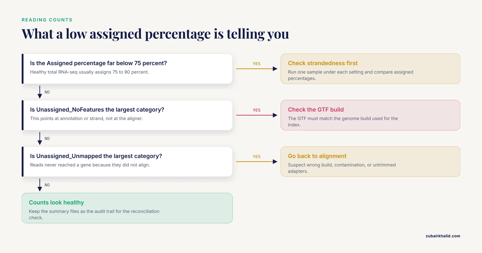
featureCounts assigns reads to genes using your GTF annotation.
- Search for featureCounts (in "RNA-seq").
- Inputs: your sorted BAM file(s) from HISAT2, and the GTF annotation matching the exact same genome build. On public servers the built-in annotation is offered in a dropdown consistent with the index you used. If the dropdown does not show your build, that is a signal you chose an unusual index.
- Parameters that decide whether your counts are correct:
- Strandedness. Choose unstranded, forward, or reverse to match your library protocol. Modern dUTP-based strand-specific protocols are usually "reverse". The wrong setting does not produce an error, it produces half or nearly zero counts, so this is the most dangerous silent failure in the whole pipeline.
- Feature type:
exon(the default and correct choice for gene-level counting). - Attribute:
gene_id(groups counts by gene rather than by individual transcript). - Output: the default gene counts table plus the summary file.
- Run on all samples, then use featureCounts' built-in summary output for a quick sanity check.
Expected summary (illustrative, for one sample):
Assigned:            1,842,301  (81.4%)
Unassigned_Unmapped:    122,150  (5.4%)
Unassigned_Ambiguity:    88,012  (3.9%)
Unassigned_NoFeatures:  165,301  (7.3%)
Roughly 75 to 90 percent assigned is a healthy range for good total RNA-seq. If you see a tiny Assigned percentage with a huge Unassigned_NoFeatures, your strandedness is wrong or your GTF does not match the genome. If you see a huge Unassigned_Unmapped, go back to the alignment step.
Step 6: Differential Expression with DESeq2
DESeq2 is the statistical workhorse that converts raw counts into a table of genes with fold changes, p values, and adjusted p values. It expects raw counts (not normalized ones) and performs its own normalization.
- Search for Differential abundance analysis with DESeq2 (exact tool name varies slightly by Galaxy version and wrapper).
- Factor levels. Create a factor, for example
condition, with levelscontrolandtreated, and assign each count file to a level. The level order defines the direction of the fold change (the second level is compared against the first). - Design formula. Enter
~ conditionfor a simple two-group comparison. If you have a batch effect, for example samples prepared on two different days, use~ batch + condition. The tilde means "model expression as a function of". Writing the batch term first lets DESeq2 absorb the day-to-day variation so it does not contaminate your condition comparison. - Execute.
Expected output table (de-tabular, one row per gene, illustrative values):
gene_id      baseMean  log2FoldChange  lfcSE   stat     pvalue      padj
Adora3       412.7     -1.234          0.221   -5.58    2.4e-08     1.9e-06
Slc6a4       87.2      -1.907          0.364   -5.24    1.6e-07     6.4e-06
Gapdh        18244.9    0.043          0.089    0.48    6.3e-01     8.9e-01
Columns, in plain terms:
- baseMean: average normalized expression across all samples.
- log2FoldChange: the effect size. A value of -1.23 means the gene's expression roughly halves under the treatment.
- lfcSE: the standard error of that log fold change.
- pvalue and padj: padj is the p value corrected for testing thousands of genes at once (false discovery rate correction). Genes are usually called differentially expressed at padj below 0.05.
The tool also produces diagnostic plots. The most instructive is the dispersion plot, which shows how variability declines with expression level, and the sample distance heatmap or PCA, which shows whether your biological groups separate. If samples cluster by batch instead of by condition in the PCA plot, your design formula is missing the batch term.
Step 7: Turn the History into a Reusable Workflow
This step is what separates a one-off analysis from a pipeline, and it takes about ten minutes.
- In the history dropdown (gear icon), choose Extract workflow.
- Galaxy builds a draft workflow from your history: every green dataset connected in the order you ran them. It automatically excludes failed steps and lets you choose which datasets to treat as workflow inputs (mark your FASTQ collection and the GTF as inputs; everything downstream follows).
- Open the workflow in the Workflow Editor. Do three things:
- Rename steps descriptively (
fastqc_pre,cutadapt,hisat2,featureCounts,deseq2). - Click each tool step and verify the parameters are the ones you validated. Any value you changed in the history should carry over, but confirm the strandedness and adapter sequence in particular.
- Add annotation in each step's "Annotation" field explaining the choice. This is documentation that travels with the workflow.
- Save. From the Workflows menu, you can now Run it: Galaxy presents a form where you attach a new FASTQ collection and the workflow executes the entire chain unattended.
To share or export:
- Share a history or workflow with specific users (email-based) or make it publicly accessible from the same share menu. A public workflow link is how tutorials like MIGHTS deliver reproducible analyses to learners, and how published method papers distribute pipelines [1][2].
- Export: workflows download as a
.gaJSON file, which can be imported into any other Galaxy instance or contributed to the Galaxy Training Network materials.
Step 8: Verify the Whole Pipeline, Not Just Each Step
Per-step checks were covered above. Three end-to-end checks catch the residual problems:
- Read numbers reconcile. Reads in (FASTQ line count divided by 4) should approximately equal reads counted plus reads unmapped plus reads dropped. Cutadapt's and featureCounts' summary files make this arithmetic easy. If you lose 30 percent of reads between two steps with no visible trimming loss, something is wrong.
- PCA or heatmap sanity. Biological replicates of the same condition should cluster together. If they do not, no downstream statistics will rescue the analysis.
- Effect direction. In DESeq2, confirm the sign of the log2FoldChange matches your biological expectation for a gene you know well. Sign errors almost always come from factor level order.
Checking Your Results Against the Literature
Once you have a differential expression table, a good habit is to compare it with published analyses of similar data. Reading how published studies structure their analyses also teaches you what a complete analysis looks like. For example, published integrative studies typically combine bulk datasets from public repositories such as GEO with machine learning feature selection, Mendelian randomization, and single-cell RNA-seq validation to identify candidate targets, with pseudotime and cell-cell communication layers added on top [3]. Your simple pipeline is the foundation those layers sit on. The counting step and the differential expression table you just produced are the same primitives those studies use, just with more samples and more comparisons.
Galaxy Bioinformatics Pipeline Tutorial Tips
These are the tips that save the most time on a second and third run.
- Build with a small dataset first. Use the GTN test history. Validate strandedness, adapter, and annotation on a fraction of the data before committing hours of compute. Then run the workflow on the full samples.
- Use dataset collections for multi-sample runs. A "list:paired" collection lets one HISAT2 step process all 12 samples in parallel instead of you filling 12 forms. Extract workflow from a history built with collections and the workflow inherits that structure.
- Keep the summary files. Cutadapt reports, HISAT2 alignment summaries, and featureCounts summaries are tiny. Keep them. They are the audit trail for the reconciliation check.
- Name inputs at the workflow level. In the workflow editor, give inputs human labels like "FASTQ R1 reads". Users who run your workflow later, including future you, see those labels in the run form.
- Annotate as you go, not after. The Galaxy annotation field on each step takes one sentence. Write it while the reasoning is fresh.
- Interleave learning materials. The MIGHTS suite demonstrates a useful pattern: the same analysis presented in both graphical and code-based form. After you finish the button version of a step, peek at the equivalent script in the training material. That pairing accelerates the transition when you eventually want to work outside Galaxy [1].
- Prefer published workflows for specialized questions. If your question is variant detection in a model organism, a purpose-built Galaxy workflow with tailored filtering and an accompanying tutorial for manual curation of the candidate list will beat a pipeline you assemble from scratch on day one [2].
Common Mistakes and Limitations
These are the mistakes that appear over and over in beginner histories, with the fix for each.
- Wrong datatype on upload. Galaxy guesses file types and sometimes guesses wrong, tagging a FASTQ as generic
fastqor even as text. Tools then fail or produce garbage. Fix: check the pencil icon attributes on every uploaded dataset and forcefastqsanger/fastqsanger.gz. - Mismatched genome build between index and GTF. Aligning against mm10 and counting against an mm9 GTF yields near-zero assigned reads. Symptom: a featureCounts summary dominated by
Unassigned_NoFeatures. Fix: use the same build everywhere, ideally by selecting both from the built-in dropdowns and confirming the build tag matches. - Wrong strandedness. The pipeline completes, the numbers look plausible, and half your gene counts are wrong. Symptom: abnormally low assigned fraction, or a PCA where samples cluster oddly. Fix: run featureCounts once per strandedness setting on one sample and compare assigned percentages. The correct setting is obvious in the summary.
- Not re-running QC after trimming. Trimming with a wrong adapter sequence changes nothing, and if you never look at post-trim FastQC you never learn that. Symptom: Adapter Content plot still climbing after Cutadapt. Fix: always run FastQC on trimmed output and compare.
- Feeding normalized counts into DESeq2. DESeq2 requires raw counts and does its own size factor normalization. Symptom: a DESeq2 error like
Error in estimateSizeFactorsForMatrix: every gene contains at least one zero, cannot compute log geometric means, or statistically absurd results. Fix: feed the featureCounts raw table, not a normalized or TPM-converted table. - Ignoring the size of the problem on public servers. Full mammalian transcriptome runs can exceed quotas and queue for a long time behind other users. Fix: test small, delete unneeded intermediates, and be patient or move to an institutional Galaxy.
- Trusting a green dataset. Green means the tool exited successfully, not that the biology is correct. The strandedness and adapter mistakes above both produce green datasets. Fix: run the verification checks in the sections above.
- Treating the pipeline as validated science on first pass. A Galaxy history reproduces your clicks. It does not validate your experimental design, replicate structure, or statistical model. Batch effects, inadequate replication, and mislabeled samples survive any tool chain intact.
Limitations worth stating plainly. Galaxy's graphical interface hides the underlying command-line invocations, so a button-only user learns analysis logic without learning to script, which limits later work on large-scale or custom analyses. Public servers impose quotas and queue times that make them unsuitable for production-scale projects. And no pipeline, however carefully built, substitutes for proper experimental design or, in any clinical or applied context, expert review of the individual case.
How to Keep Learning Bioinformatics with Galaxy
The pipeline above is deliberately minimal. The Galaxy Training Network hosts a structured curriculum that extends it in every direction, and it is the standard entry point for people who want to learn bioinformatics without first learning to program. The MIGHTS project is a good model of how that learning works best: parallel graphical and code-based tracks, real datasets rather than toy examples, and materials built on FAIR data principles so learners can validate their results against known answers [1].
Structured, hands-on exposure works. In one assessment of a course-based undergraduate research experience spanning five semesters and more than 300 students, 96 percent of students reported an increase in bioinformatics techniques as an anticipated learning outcome, and more than 90 percent reported gains in knowledge, experience, and confidence [4]. The lesson generalizes: bioinformatics skills consolidate when you apply them to a real question with real data, which is exactly what rerunning your new workflow on a dataset you care about accomplishes.
A practical progression:
- Rerun this workflow on a dataset from your own field.
- Follow one GTN tutorial per week in a new domain (variant calling, single-cell, metagenomics).
- Compare your history's command log with the equivalent script in the training material to start picking up the code layer.
- Contribute back: export your workflow, annotate it, and share it publicly, the same way published workflows like MOM are distributed with tutorials and curation guidelines [2].
Frequently Asked Questions
Do I need to know how to program to build a pipeline in Galaxy?
No. Galaxy's entire workflow, from upload to workflow extraction, runs through web forms and menus. Programming helps when you eventually want to customize beyond the available wrappers, and Galaxy's training materials deliberately support a transition from buttons to code [1].
Which Galaxy server should I use?
Any of the main public servers, usegalaxy.org, usegalaxy.eu, or usegalaxy.org.au, will run this pipeline. Pick the one nearest to you for lower latency and check which holds the built-in genome indices you need.
How much data can a public Galaxy server handle?
Registered users get a fixed disk quota and fair-share compute limits that are fine for tutorials and moderate projects. For a full 12-sample mammalian RNA-seq project, expect to manage intermediate files carefully or use an institutional or self-hosted Galaxy.
How do I know if my alignment rate is acceptable?
For a clean mammalian total RNA-seq library, an overall alignment rate in the high 80s to mid 90s percent range is typical. A much lower rate usually means the wrong genome build, contamination, or a problem in the input reads, not a tool failure.
Why is strandedness so important in the counting step?
If featureCounts is set to the wrong strandedness, reads get assigned to the wrong strand and most gene counts collapse toward zero or become nonsensical, without any error message. Run one sample under each setting and compare the assigned percentages to find the correct one.
Can I use Galaxy pipelines for single-cell RNA-seq?
Yes. Single-cell analysis is an area of active Galaxy development and training, and the MIGHTS suite provides complete graphical and code-based training tracks for scRNA-seq on the Galaxy Training Network [1].
What file formats does this pipeline use?
FASTQ for raw reads, BAM for alignments, GTF for gene annotation, tabular text for count matrices and the DESeq2 results table, and HTML for QC reports. All are visible and downloadable from the history.
How do I share my finished pipeline with a collaborator?
Use the "Share or publish" option on your history or workflow. You can share by email with specific Galaxy users, make it publicly accessible with a link, or export the workflow as a .ga file that any Galaxy instance can import.
Further Reading
- Impact of training data on deep learning-based RNA 3D structure quality assessment.
- Adaptive causal discovery with ordering-based reinforcement learning-approach for type 2 diabetes mellitus risk factors.
Sources
- Galaxy as a gateway to bioinformatics: Multi-Interface Galaxy Hands-on Training Suite (MIGHTS) for scRNA-seq.
- Model Organism Modifier (MOM): a user-friendly Galaxy workflow to detect modifiers from genome sequencing data using Caenorhabditis elegans.
- Bioinformatics Analysis to Reveal Potential Targets of Huntington's Disease.
- Analysis of Perceived Student Learning Gains in a Biochemistry Lab Course-Based Undergraduate Research Experience.