How to Run Functional Enrichment Analysis on a Gene List in R

By Dr. Zubair Khalid, DVM, MS, PhD · 2026-11-11

By the end of this walkthrough you will be able to take a differential expression table from DESeq2, format it correctly, run over-representation analysis (ORA) and gene set enrichment analysis (GSEA) with clusterProfiler, and produce figures that hold up in a paper or thesis. You will also know how to define a background universe, convert gene identifiers, read every column of the output, reproduce a p-value by hand, and fix the errors that stop most first attempts.

Have the following on hand before you start: R 4.3 or newer, the packages installed in Step 1, a raw count matrix with genes in rows and samples in columns, and a sample metadata table. Everything runs in a local R session. No server, cluster, or cloud account is required.

Functional enrichment analysis is the standard bridge between a list of differentially expressed genes and a biological interpretation. Current methods literature describes it as a cornerstone of transcriptomics and proteomics analysis, and clusterProfiler is one of its most widely used implementations, combining robust statistics with bar plots, dot plots, and network visualizations [1].

What Functional Enrichment Analysis Does

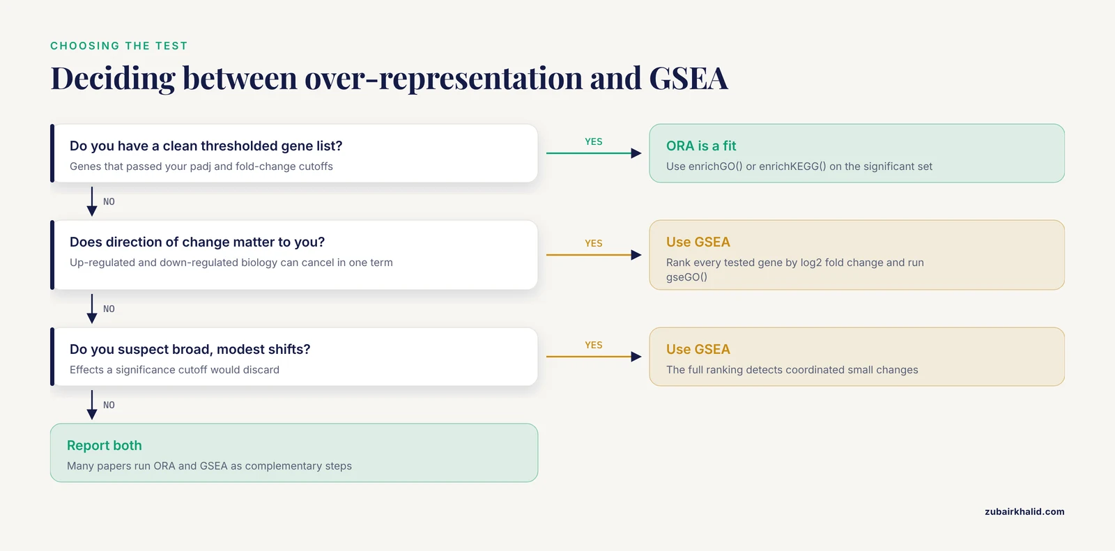
Over-representation analysis (ORA) answers a narrow question. Given my list of significant genes, does any Gene Ontology (GO) term or pathway contain more of them than expected by chance? The underlying test is the hypergeometric distribution, which is equivalent to Fisher's exact test on a two-by-two table of counts. The Gene Ontology is a controlled vocabulary of gene functions organized into three branches: biological process (BP), molecular function (MF), and cellular component (CC). KEGG, the Kyoto Encyclopedia of Genes and Genomes, maps genes to signaling and metabolic pathways.

Gene set enrichment analysis (GSEA) takes a different input. Instead of a thresholded list, it uses every tested gene ranked by a statistic, usually the log2 fold change, and walks down the ranking looking for gene sets that cluster toward the top or the bottom. Because it uses the full ranking, it detects coordinated modest shifts that a significance cutoff would discard.

Both approaches belong in the same analysis. Quantitative proteomics pipelines treat ORA and GSEA as standard, complementary steps after differential testing [2], and the same logic holds for RNA-seq. The gene-list format also extends beyond expression data. A large bladder cancer GWAS meta-analysis used pathway enrichment of prioritized genes to implicate xenobiotic metabolism [3], and metabolomics methods chapters build interpretation around enrichment against prior knowledge databases [4].

A practical decision rule: use ORA when you have a clean thresholded list and want the fastest route to interpretable terms. Use GSEA when direction matters or when you suspect broad, modest shifts. Many papers report both.

The Functional Enrichment Workflow in R: From DESeq2 to clusterProfiler

The complete functional enrichment workflow in R with DESeq2 and clusterProfiler has seven steps:

1. Install R, Bioconductor, and the required packages.
2. Run DESeq2 and extract a results table.
3. Convert gene identifiers to Entrez IDs.
4. Define the background universe.
5. Run over-representation analysis with enrichGO() and enrichKEGG().
6. Run GSEA with gseGO() and gseKEGG().
7. Visualize, simplify, and export the results.

Two input formats drive everything. ORA wants a character vector of Entrez IDs, optionally with a universe vector of the same type. GSEA wants a named numeric vector where the names are Entrez IDs, the values are log2 fold changes, and the vector is sorted from most positive to most negative. Nearly every error you will hit in this workflow traces back to one of those two formats being wrong.

Step 1: Install R, Bioconductor, and the Required Packages

Most packages used in R for bioinformatics live on Bioconductor, the official repository for genomic analysis software. Install its manager first, then the packages:

install.packages("BiocManager")
BiocManager::install(c(
  "DESeq2",
  "clusterProfiler",
  "org.Hs.eg.db",
  "enrichplot",
  "apeglm"
))
install.packages("msigdbr")  # optional, MSigDB gene sets for custom analyses

Bioconductor pins package versions to your R version. If BiocManager reports that the current Bioconductor release requires a newer R, update R first and reinstall. Mixing an old R with a forced Bioconductor version produces dependency errors that are tedious to unwind.

Confirm the installation and record your environment:

library(DESeq2)
library(clusterProfiler)
library(org.Hs.eg.db)
library(enrichplot)
packageVersion("clusterProfiler")
sessionInfo()

Two errors appear constantly at this stage. could not find function "DESeqDataSetFromMatrix" means DESeq2 is installed but not attached, so run library(DESeq2). object 'org.Hs.eg.db' not found means the annotation database is installed but not attached, so run library(org.Hs.eg.db).

Step 2: Produce a Differential Expression Table with DESeq2

DESeq2 estimates differential expression from raw RNA-seq counts using a negative binomial model. The example below uses a two-group design with a condition factor. For batched experiments, extend the design to ~ batch + condition.

cts     <- read.csv("counts.csv",  row.names = 1)  # genes in rows, samples in columns
coldata <- read.csv("coldata.csv", row.names = 1)  # rownames must match colnames(cts)

dds <- DESeqDataSetFromMatrix(countData = round(cts),
                              colData   = coldata,
                              design    = ~ condition)

dds$condition <- relevel(factor(dds$condition), ref = "control")
dds <- dds[rowSums(counts(dds)) >= 10, ]   # standard pre-filter for near-empty rows
dds <- DESeq(dds)
resultsNames(dds)

The round() call matters if your counts came through tximport from Salmon or kallisto, because DESeq2 requires integers. The pre-filter drops genes with fewer than 10 total reads across all samples, which removes noise rows without affecting the model.

Expected output of resultsNames(dds):

[1] "Intercept"                    "condition_treated_vs_control"

Extract the results and apply fold-change shrinkage:

res <- results(dds, contrast = c("condition", "treated", "control"), alpha = 0.05)
res <- lfcShrink(dds, coef = "condition_treated_vs_control",
                 type = "apeglm", res = res)
head(res)

Illustrative output from results() (your numbers will differ):

log2 fold change (MLE): condition treated vs control
Wald test p-value: condition treated vs control
DataFrame with 6 rows and 6 columns
       baseMean log2FoldChange     lfcSE      stat      pvalue        padj
      <numeric>      <numeric> <numeric> <numeric>   <numeric>   <numeric>
GENE01   1254.7         2.4130    0.3012    8.0112 1.2e-15     4.3e-12
GENE02    812.9        -1.8770    0.2871   -6.5378 6.2e-11     1.1e-08
GENE03    309.4         1.6420    0.3348    4.9044 9.4e-07     9.8e-05

The columns are baseMean (average normalized count), log2FoldChange, lfcSE (its standard error), stat (Wald statistic), pvalue, and padj (the Benjamini-Hochberg adjusted p-value, your false discovery rate). Shrinkage with apeglm updates the log2FoldChange and lfcSE columns while keeping the p-values. The Wald statistic is not the quantity to read after shrinkage, so base your thresholds on padj and the shrunk fold change. Note that results() uses alpha = 0.1 by default for its independent filtering step, so pass alpha = 0.05 when your cutoff is 0.05.

Build the significant set you will test:

res_df <- as.data.frame(res)
res_df$symbol <- rownames(res_df)
sig_df <- subset(res_df, padj < 0.05 & abs(log2FoldChange) > 1)
nrow(sig_df)

This example assumes gene symbols as rownames, which is common with featureCounts output. If your counts carry Ensembl IDs, keep them and use fromType = "ENSEMBL" in Step 3 instead.

Step 3: Convert Gene Identifiers to Entrez IDs

The GO and KEGG mappings inside organism annotation databases are keyed by Entrez IDs, the numeric gene identifiers maintained by NCBI. clusterProfiler accepts other key types for GO, but Entrez is the safest common currency, and KEGG effectively requires it.

sig_ids <- bitr(sig_df$symbol,
                fromType = "SYMBOL",
                toType   = "ENTREZID",
                OrgDb    = org.Hs.eg.db)
nrow(sig_ids)
nrow(sig_df)

bitr() uses the org.Hs.eg.db annotation package (the human OrgDb, short for organism database) to convert identifiers. Expect a warning like this:

Warning message:
In bitr(...) : 3% of input gene IDs are fail to map...

A few percent failing is normal. A large failure rate means the wrong fromType or an outdated annotation database. Every unmapped gene is silently removed from the analysis, so report the mapping rate in your methods section. Compare nrow(sig_ids) with nrow(sig_df) every time.

For Ensembl input, switch to fromType = "ENSEMBL". For genomes without an OrgDb, map through orthology. The ShEnrich platform for penaeid shrimp, for example, built its annotations from BLASTP against the NCBI nr database, InterProScan domain prediction, and eggNOG-mapper orthology assignments, then ran GO and KEGG enrichment through clusterProfiler using custom gene set files [5]. Step 7 shows how to use such custom sets with enricher().

Step 4: Define the Background Universe

ORA asks whether your genes appear in a term more often than expected. Expected relative to what? To the background universe, the set of genes that had a genuine chance of appearing in your experiment. If you omit the universe, clusterProfiler defaults to every gene annotated in the OrgDb, which includes thousands of genes your RNA-seq library never observed. That inflates significance for terms packed with well-annotated housekeeping genes and is one of the most common defects in published enrichment figures.

tested   <- res_df[!is.na(res_df$padj), ]   # genes that survived the test
universe <- bitr(tested$symbol, fromType = "SYMBOL", toType = "ENTREZID",
                 OrgDb = org.Hs.eg.db)$ENTREZID
universe <- unique(universe)
length(universe)

Using genes with a non-NA padj is a defensible default because those are the genes DESeq2 actually tested to completion. Two rules apply. The universe must use the same ID type as your gene list. And your gene list must be a subset of it. If some significant genes vanish during universe mapping, the overlap logic breaks quietly, so compare vector lengths before and after.

Step 5: Run Over-Representation Analysis

GO over-representation with enrichGO()

ego <- enrichGO(
  gene          = sig_ids$ENTREZID,
  universe      = universe,
  OrgDb         = org.Hs.eg.db,
  keyType       = "ENTREZID",
  ont           = "BP",
  pAdjustMethod = "BH",
  pvalueCutoff  = 0.05,
  qvalueCutoff  = 0.05,
  readable      = TRUE
)
head(as.data.frame(ego)[, c("ID","Description","GeneRatio",
                            "BgRatio","pvalue","p.adjust","Count")])

Each parameter does one job. gene is your character vector of Entrez IDs. universe is the background from Step 4. OrgDb is the annotation database object. keyType declares the ID type of both gene and universe. ont selects the branch, with "BP" the usual starting point and "MF" and "CC" worth running separately. pAdjustMethod = "BH" applies Benjamini-Hochberg correction and is the right default. pvalueCutoff and qvalueCutoff filter the result table. readable = TRUE converts the geneID column back to symbols for readability.

Expected output (illustrative, your values will differ):

          ID       Description                      GeneRatio BgRatio     pvalue  p.adjust Count
1 GO:0006412 translation                       18/402     180/11980  6.1e-05  0.0031   18
2 GO:0009410 response to xenobiotic stimulus   12/402      95/11980  1.4e-04  0.0048   12
3 GO:0006096 glycolytic process                12/402     132/11980  1.9e-04  0.0052   12

GeneRatio 18/402 means 18 of your 402 mapped significant genes belong to the term. BgRatio 180/11980 means 180 of the 11,980 universe genes are annotated to it.

A worked p-value you can reproduce

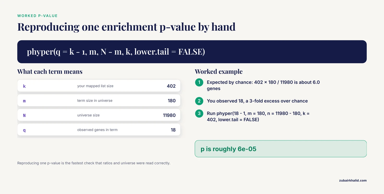
Expected by chance: 402 × 180 / 11,980 ≈ 6.0 genes. You observed 18, a 3-fold excess. clusterProfiler computes the exact hypergeometric tail, and you can reproduce any single row yourself:

phyper(18 - 1, m = 180, n = 11980 - 180, k = 402, lower.tail = FALSE)
# roughly 6e-05 for these numbers

Here m is the term size in the universe, n is the universe minus the term, and k is your list size. Reproducing one p-value by hand is the fastest sanity check that the ratios and universe were interpreted the way you think they were.

KEGG pathway over-representation with enrichKEGG()

ekk <- enrichKEGG(
  gene          = sig_ids$ENTREZID,
  universe      = universe,
  organism      = "hsa",
  pAdjustMethod = "BH",
  pvalueCutoff  = 0.05
)
ekk <- setReadable(ekk, OrgDb = org.Hs.eg.db, keyType = "ENTREZID")

enrichKEGG() queries the KEGG REST API over the internet, so it fails with download errors when offline. KEGG gene identifiers for human are Entrez-style IDs, which is why Step 3 matters here. KEGG has license terms that restrict systematic and commercial use, so check them for your project type.

Step 6: Run Gene Set Enrichment Analysis on the Ranked List

Build the ranked vector

all_ids <- bitr(res_df$symbol, fromType = "SYMBOL", toType = "ENTREZID",
                OrgDb = org.Hs.eg.db)
ranked  <- merge(all_ids, res_df, by.x = "SYMBOL", by.y = "symbol")
ranked  <- ranked[!duplicated(ranked$ENTREZID), ]

geneList <- ranked$log2FoldChange
names(geneList) <- ranked$ENTREZID
geneList <- sort(geneList[!is.na(geneList)], decreasing = TRUE)
head(geneList, 3)

Expected output:

     1234      5678      9012
4.213027  3.918412  3.544201

Three hard requirements: every element named with an Entrez ID, no NA values, sorted decreasing. clusterProfiler stops with an error if the vector contains NA or arrives unsorted, and the fix is always the same, drop NA with geneList[!is.na(geneList)] and sort with decreasing = TRUE. Do not pre-filter this vector to significant genes. The entire point of GSEA is to use every tested gene, and pre-filtering makes the test circular.

gseGO() and gseKEGG()

egse <- gseGO(
  geneList     = geneList,
  ont          = "BP",
  OrgDb        = org.Hs.eg.db,
  keyType      = "ENTREZID",
  minGSSize    = 15,
  maxGSSize    = 500,
  pvalueCutoff = 0.05,
  verbose      = FALSE
)
head(as.data.frame(egse)[, c("ID","Description","setSize","NES","pvalue","p.adjust")])

Illustrative output:

          ID       Description        setSize    NES   pvalue  p.adjust
1 GO:0006412 translation          312     2.41   0.001    0.011
2 GO:0006096 glycolytic process   156     1.94   0.003    0.024

NES is the normalized enrichment score, the raw enrichment score scaled against the null distribution. Positive NES means the set sits toward the top of your ranking, the up-regulated end. Negative NES means the bottom. minGSSize and maxGSSize keep tiny, unstable sets and sprawling catch-all terms out of the results, and 15 to 500 is a sensible window for GO.

ekegg <- gseKEGG(geneList     = geneList,
                 organism     = "hsa",
                 minGSSize    = 15,
                 pvalueCutoff = 0.05)

Set a random seed before running GSEA if you need exactly reproducible p-values across sessions, and record the seed together with sessionInfo() in your methods.

Step 7: Visualize, Simplify, and Export the Results

Standard plots

dotplot(ego, showCategory = 20)
cnetplot(ego, showCategory = 10)
ridgeplot(egse, showCategory = 20)

The dot plot is the workhorse figure, with GeneRatio on one axis and the adjusted p-value encoded in dot size or color. The category network plot shows genes shared between terms. The ridge plot shows where the genes of each GSEA hit fall along your ranking.

Enrichment maps and Cytoscape

GO is redundant, parent and child terms overlap heavily, so a raw GO table often shows five versions of the same biology. simplify() collapses terms by semantic similarity:

ego_sim <- simplify(ego, cutoff = 0.7)
emapplot(ego_sim, showCategory = 30)

Enrichment maps draw terms as nodes connected by shared gene content, which turns a 40-row table into a picture of functional modules. The current reference protocol for clusterProfiler visualization goes further, computing term similarity and exporting the network to Cytoscape with the cyemapplot function, where node properties can encode pathway coverage and expression directionality [1]. Start Cytoscape before running the export, because the handoff communicates through the CyREST interface.

Split by direction with compareCluster()

ORA pools up-regulated and down-regulated genes, which can cancel opposing biology inside one term. Splitting by sign is the cheapest fix:

sig_full  <- merge(sig_ids, sig_df, by.x = "SYMBOL", by.y = "symbol")
up_ids    <- sig_full$ENTREZID[sig_full$log2FoldChange > 0]
down_ids  <- sig_full$ENTREZID[sig_full$log2FoldChange < 0]

ck <- compareCluster(
  list(up = up_ids, down = down_ids),
  fun          = "enrichGO",
  OrgDb        = org.Hs.eg.db,
  ont          = "BP",
  pvalueCutoff = 0.05
)
dotplot(ck)

This one call runs ORA on each list and returns a single object that dotplot() renders as a side-by-side figure, which also works as a reusable template for multi-contrast experiments.

Custom gene sets and non-model organisms

term2gene <- read.csv("my_pathways.csv", col.names = c("term", "gene"))
ecustom <- enricher(sig_ids$ENTREZID, TERM2GENE = term2gene,
                    universe = universe, pvalueCutoff = 0.05)

enricher() and GSEA() accept any term-to-gene mapping as a two-column data frame, which is the format behind GMT files, MSigDB sets (available through the msigdbr package, check its argument names in your installed version since they changed between releases), and species-specific pathway libraries. This is how non-model organisms get enrichment analysis at all, as the shrimp platform built on clusterProfiler demonstrates [5].

Sanity checks before you trust the table

1. Reproduce one p-value with phyper() as shown in Step 5.
2. Confirm the GeneRatio denominator equals your mapped list size and the BgRatio denominator equals your universe size.
3. Confirm the top terms match known biology of your system. Enrichment results earn trust when they line up with independent evidence. A transcriptomics study of deltamethrin resistance in Aedes aegypti found cytochrome P450 terms and xenobiotic metabolism KEGG pathways enriched among up-regulated genes, consistent with detoxification biology and validated by qPCR [6]. Proteomic comparisons of breast cancer xenograft models used enrichment to surface lipid metabolism programs shared across species [7], and a genome-wide analysis of conserved human intronic regions mapped to RNA processing and chromatin remodeling genes [8].
4. Save the result objects with saveRDS() and archive sessionInfo() output.

Sensible next steps after this pipeline: run compareCluster() across time points or multiple contrasts, add MSigDB hallmark sets through enricher(), and export the enrichment network to Cytoscape for interactive exploration [1].

Key clusterProfiler Functions and Parameters

Common Mistakes and Limitations

1. Using the default universe for RNA-seq. Without universe, ORA compares your list against every gene in the annotation database, including genes your library never sampled. Always pass the tested set from Step 4.

1. Feeding the wrong ID type. Passing gene symbols while keyType = "ENTREZID" produces the message No gene can be mapped, followed by the expected ID type. Either convert with bitr() or change keyType to match your vector.

1. Ignoring silent gene loss. bitr() drops unmapped genes with only a warning. If 20 percent of your list fails to map, your enrichment questions a different list than the one you built. Report the mapping rate.

1. Running GSEA on a pre-filtered list. Thresholding before GSEA removes the modest coordinated shifts the method exists to detect and makes the ranking uninformative. Save thresholds for ORA.

1. Leaving NA fold changes in the ranked vector. DESeq2 returns NA for some low-count and outlier genes. GSEA refuses NA input, so filter with geneList[!is.na(geneList)] before sorting.

1. Reporting redundant GO terms. Parent and child terms inflate the apparent number of findings. Run simplify() before making final figures.

1. Pooling up and down genes in one ORA. A term can be genuinely enriched because up genes pile in while down genes pile out, or the reverse. Split by sign with compareCluster() or rely on GSEA, which is direction-aware by construction.

1. Expecting enrichment from a handful of DEGs. Conventional pathway enrichment needs enough genes to detect excesses. In a reanalysis of PFAS-exposed human liver spheroids, enrichment recapitulated known SREBF- and PPAR-driven lipid metabolism effects for compounds with many DEGs but gave limited insight for PFBS, which had fewer DEGs, and the authors needed multimodal integration to recover compound-specific mechanisms [9]. If your contrast yields few DEGs, expect thin enrichment and lean on GSEA or additional data types.

1. Reading raw p-values. With thousands of terms tested, raw p-values guarantee false positives. Report p.adjust, and treat terms that survive correction as the result set.

1. Treating enrichment as mechanism. Enrichment is associative. It says a term is over-represented, not that the pathway is causally driving your phenotype. Validate top terms with independent data, and remember that upstream artifacts propagate. A single-cell proteomics study of pancreatic islet cells found that enzymatic digestion itself shifts expression patterns, especially for membrane-associated proteins [10]. If the input list is biased, the enriched terms describe the bias.

1. Skipping reproducibility records. GSEA involves stochastic p-value estimation, so record your seed, package versions, and sessionInfo() output with the analysis.

Frequently Asked Questions

Should I run ORA on all DEGs or only the significant ones?

ORA works on your thresholded list, that is the design of the test, so use the genes that passed your padj and fold-change cutoffs. GSEA is the method that uses the full ranked list, so keep thresholds out of that input.

Can I use gene symbols instead of Entrez IDs?

For GO analysis, yes, set keyType = "SYMBOL" and supply a matching symbol universe. For KEGG, convert to Entrez IDs first, because enrichKEGG() and gseKEGG() expect Entrez-style identifiers and symbol input produces empty or misleading results.

What is the difference between p.adjust and qvalue in the output?

Both estimate the false discovery rate. p.adjust uses the Benjamini-Hochberg method, while qvalue uses Storey's method with an estimated null proportion. Report p.adjust, which matches the FDR convention most reviewers expect.

Why does enrichGO tell me "No gene can be mapped"?

Your input IDs do not match the keyType argument. The message names the expected ID type, so either convert your vector with bitr() or change keyType to match what you actually have.

Do I need a universe for GSEA?

No. GSEA uses every gene in the ranked vector, so the background concept is built into the method rather than supplied as a separate argument.

How many genes does enrichment analysis need?

There is no hard minimum, but very small lists give unstable results and few DEGs limit what conventional enrichment can reveal. With a handful of DEGs, expect thin ORA output and prefer GSEA on the full ranking or integration with other data types.

What does NES mean in GSEA output?

NES is the normalized enrichment score, the enrichment score scaled against the null distribution. Positive values mean the gene set is enriched at the top of your ranked list, negative values at the bottom.

Can clusterProfiler analyze non-model organisms?

Yes, through enricher() and GSEA() with a TERM2GENE table mapping terms to genes. Build that table from orthology-based annotation, which is how recent non-model enrichment platforms were constructed.

Sources

1. Enhancing Interpretation of Functional Enrichment Analysis Results with Advanced Network Visualizations.
2. Computational and Statistical Framework for Quantitative Proteomics Analysis.
3. Multi-population GWAS meta-analysis identifies bladder cancer susceptibility loci and highlights genetic regulation of smoking-related risk.
4. Multi-Omics Guided Pathway and Network Analysis of Clinical Metabolomics and Proteomics Data.
5. ShEnrich: a functional annotation database and enrichment platform for penaeid shrimp.
6. Transcriptome Analysis of Deltamethrin Resistance Mechanisms in Aedes aegypti Populations from Metro Manila, Philippines.
7. Host-Derived Proteomic Profiling of Human and Canine Mammary Tumor Xenografts Identifies Enrichment of Lipid Metabolism-Related Pathways.
8. A genome-wide functional analysis of conserved intronic regions reveals essential roles for speckle-associated retained introns.
9. Multimodal cheminformatic and network biology analysis enables deeper mechanistic understanding of PFAS-induced hepatotoxicity.
10. Proteomic analysis of pancreatic endocrine cells by mechanistic single-cell isolation identifies membrane pathways.