Interpreting Results from Federated Multi-Omics Analyses
By Dr. Zubair Khalid, DVM, MS, PhD ·

Federated multi-omics analysis is the joint statistical analysis of genomic, transcriptomic, proteomic, metabolomic, or similar data layers that stay physically distributed across sites, cohorts, or cloud environments rather than being merged into one file. Interpreting its results means deciding which reported associations, embeddings, and integrated features reflect biology and which reflect technical differences between the contributing datasets, above all batch effects.
This skill matters because large-scale biology has moved to a model where data are generated continuously at many centers and analyzed on shared cloud infrastructure. Projects such as All of Us generate genetic data for over one million individuals and process fluctuating workloads of up to 9,000 whole-genome sequencing samples per month on AWS-based infrastructure [1]. When analyses span that many sources, the assumptions you would quietly make in a single-lab study no longer hold. A variant, protein, or metabolite that appears significant may be a discovery, or it may be a shadow cast by the machine, reagent lot, protocol version, or cohort composition that produced the data. Reading these results critically is now a core competence rather than an optional refinement.
What Does Federated Multi-Omics Interpretation Batch Effects Mean?
The phrase bundles three ideas that you have to hold at once.
Federated describes the data architecture. Raw data remain at their source, whether that is a hospital server, a national Trusted Research Environment (TRE), or a cloud bucket, and only aggregates, model updates, or summary statistics move between sites. This is common because genomic data are large, identifiable, and governed by consent terms that often restrict copying.
Multi-omics describes the data types being combined. A single study may pair genotypes with RNA-seq counts, proteomics intensities, metabolite abundances, or microbiome profiles. Each layer has its own noise structure, dimensionality, and processing pipeline.
Batch effects describe systematic, non-biological differences between groups of samples processed together. Two sequencing runs, two mass spectrometry platforms, or two cohorts with different sample prep protocols will produce measurable differences even if the underlying biology is identical. In multi-omics integration reviews, batch effects, high dimensionality, and structural heterogeneity are named as the fundamental analytical challenges of the field [2]. In single-cell multimodal work, the same list appears as batch effects, sparsity, and modality alignment [3].
So "federated multi-omics interpretation batch effects" refers to the practice of reading results from federated multi-omics studies with specific attention to whether batch effects, cohort structure, and platform differences could explain what you see. When a paper reports that a metabolite signature predicts disease across three cohorts, the interpretation question is not only "is the signal strong" but "would this signal survive if each cohort had been processed identically."
Federated Versus Pooled Analysis: Why the Same Question Gives Different Answers
A concrete study shows how much the analysis design itself changes the result. Deflaux and colleagues compared two ways of running a genome-wide association study (GWAS) of standard lipid measures across large cloud-hosted cohorts such as All of Us and the UK Biobank, both stored in cloud-based TREs [4].
The two approaches were:
- Meta-analysis. Each cohort runs the GWAS locally on its own data. The summary statistics (effect estimates and standard errors per variant) are then combined across cohorts.
- Pooled analysis. Genotype-level data are harmonized and analyzed together as a single dataset within the shared environment.
Both approaches recovered known lipid loci, with correlations of R² around 83 to 97 percent against an external reference study [4]. But the agreement was not perfect at the level of individual discoveries. Ninety variants met the significance threshold only in the meta-analysis, and sixty-four variants were significant only in the pooled analysis. Roughly 20 percent of the variants in each of those groups were most prevalent in individuals of non-European, non-Asian ancestry [4].
For interpretation, this carries a specific lesson. When you read a federated result, you are reading the output of a design decision, not a unique ground truth. Technical and policy choices, such as which cohorts can share raw data and which must exchange only summaries, lead cross-cohort analyses to generate similar but not identical results, particularly for non-European ancestral populations [4]. A variant significant in one design and not the other is not automatically false. It may reflect allele frequency differences, ancestry composition, imputation quality, or cohort-specific batch effects, and your job is to name which of those is plausible before you accept or reject the finding.
The Cloud Infrastructure Behind the Results
Interpreting federated results also requires understanding where the computation happened, because the infrastructure constrains what can be computed and therefore what appears in the tables you read.
Serverless, containerized pipelines. Celeste, the open-source cloud architecture behind All of Us genomics, runs on AWS and uses serverless technology and container orchestration to manage population-scale sequencing. In 12 months of production within a single AWS Region, around 200 million serverless functions and over 20 million messages coordinated 1.8 million bioinformatics, quality control, and clinical reporting jobs [1]. When you interpret a variant call from such a system, you are interpreting the end point of a massively distributed pipeline. Pipeline version, workflow parameters, and the specific queue a job ran in are part of the batch structure of the data, and they belong in your interpretation.
Distributed machine learning. VariantSpark is a cloud-based machine learning framework for association studies that searches for epistatic interactions, the combined effects of variants that do not show additive effects alone. It scales to datasets with 100,000,000 genomic variants and 100,000 samples and runs 3.6 times faster than ReForeSt while being the only method of the two able to handle that dimensionality in manageable time [5]. Results from such random-forest-based association methods look different from GWAS tables. Instead of a per-variant p-value row, you may get feature importance scores or pairwise interaction strengths. Interpreting them means remembering that importance measures ranking, not effect direction, and that hyperparameters and data partitioning across a cluster are part of the method's behavior.
Interactive columnar databases. A different paradigm replaces batch jobs with interactive queries. Pan and colleagues demonstrated cloud-based interactive analytics for terabytes of variant data using a columnar database built on Dremel, implemented in Google Cloud Platform BigQuery, applied to a study population of 475 deeply sequenced human genomes to assess genomic call rate, genotype and allele frequency distributions, variant density, and pharmacogenomic information [6]. This matters for interpretation because it changes the workflow. Quality control becomes a question you ask from a web browser in seconds rather than a long-running shell job [6], which makes it practical to interrogate batch structure directly before trusting any downstream result.
Workflow wrappers that lower the barrier. AnVILWorkflow is an R package that lets researchers run bioinformatics workflows hosted on the AnVIL platform, covering use cases such as bulk RNA-seq analysis with Salmon, metagenomics with bioBakery, and digital pathology with PathML [7]. Convenience cuts both ways in interpretation. A package that handles environment setup, data formatting, submission, and retrieval for you [7] can also make it tempting to accept default parameters. Defaults chosen for one data type or one batch structure may be wrong for yours.
AWS genomics in context. When an article mentions aws genomics, it typically refers to this family of services, including serverless orchestration and container orchestration of the kind Celeste uses [1], plus scalable storage and query layers. Cloud bioinformatics more broadly covers the TRE model used by All of Us and the UK Biobank [4], interactive query engines [6], and workflow platforms accessible from R [7]. Knowing which model produced your result tells you which artifacts to look for.
Batch Effects Explained
A batch effect is a systematic difference in measured values that tracks with processing group rather than biology. The classic examples in genomics are sequencing center, library preparation kit, flow cell, and read depth. In proteomics and metabolomics, they include instrument calibration drift, reagent lots, and acquisition order. In spatial omics, slide, capture area, and segmentation algorithm version all act as batches, and batch-effect correction is listed among the core computational tasks for the field alongside cell segmentation and spatial domain discovery [8].
Three properties make batch effects dangerous in federated multi-omics work.
They can be larger than biological effects. If cohort A ran on one platform and cohort B on another, the strongest axis of variation in the combined data may separate the cohorts rather than the phenotypes. In a federated design where each site's data never leave the site, you often cannot see this directly, because no one ever plots the merged raw data.
They correlate with real covariates. Sites enroll different populations. The Deflaux cross-cohort study showed that variants unique to one analysis design were enriched for variants most prevalent in non-European, non-Asian ancestry individuals [4]. In that case the difference came from analysis design rather than chemistry, but the same logic applies to technical batches. If a processing change coincided with a change in recruitment, the batch effect and the ancestry signal are entangled, and standard correction tools can remove real signal along with the artifact.
Correction methods have assumptions. Deep learning methods, including variational autoencoders and graph neural networks, are now standard tools for harmonizing omics layers and improving feature extraction in single-cell multimodal integration, with tools such as sciCAN, scJoint, and scMaui representing the approach [3]. In chemometrics-driven multi-omics integration, convolutional neural networks, autoencoders, variational autoencoders, and graph neural networks perform non-linear feature extraction and data fusion [2]. These models learn latent representations in which batch and biology are supposed to disentangle. Whether they actually do depends on the experimental design. If batch is confounded with phenotype, meaning every case was processed in batch one and every control in batch two, no algorithm can separate them, because the information required does not exist in the data. Reviewers of these methods flag model interpretability, scalability, and generalizability across datasets as persistent open problems [3], and scalability, overfitting, and validation gaps as persistent challenges [2].
How Batch Effects Interact with Federated Analysis
In a conventional pooled study, batch effects are handled by randomizing samples across batches and applying correction methods such as linear modeling on the merged matrix. Federated designs remove some of those options and add others.
What you lose. You generally cannot re-randomize samples across sites, because the sites are fixed by consent and geography. You may not be able to apply harmonization algorithms that require access to joint raw data, since raw data stay local.
What you gain. Site-level analysis gives you a natural replicate structure. If a signal appears consistently within every site's internal analysis, where each site's data are internally homogeneous, it is less likely to be a between-site batch artifact. This is one reason the meta-analysis arm of the cross-cohort lipid study found 90 significant variants that the pooled arm did not [4]. Design-dependent differences are information, not just noise.
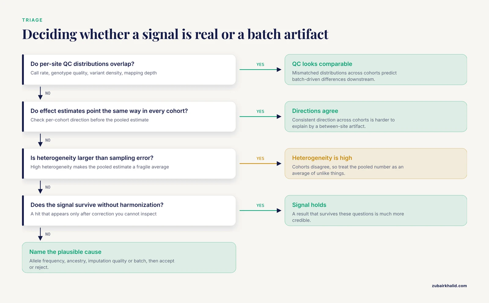
Practical checks you can request or run. Within a TRE, per-site quality metrics such as genomic call rate and allele frequency distributions can be computed and compared interactively, as demonstrated on 475 deeply sequenced genomes using a Dremel-based columnar backend [6]. For a federated multi-omics result, the analogous questions are:
- Are per-site QC distributions overlapping or disjoint?
- Do effect estimates point in the same direction in every cohort?
- Is heterogeneity across cohorts larger than expected from sampling error alone?
- Does the signal hold within the subset of samples processed under each protocol version?
- Were any normalization steps applied per site before aggregation, and are they documented?
A result that survives those questions is much more credible than one that appears only after a harmonization step you cannot inspect.
Reading the Outputs Step by Step
Most federated multi-omics papers and reports share a common set of output types. Here is how to work through them.
Step 1: Start with the cohort and pipeline description
Before any p-value, establish which cohorts contributed, how many samples from each, which pipeline versions processed each data layer, and when. A system like Celeste processed 1.8 million jobs in 12 months [1], which means pipeline code and parameters evolved during the study window. Ask whether results were generated under a single frozen version or across versions. Results spanning versions carry version as a potential batch variable.
Step 2: Read the quality control summary before the discovery table
Per-cohort QC metrics are your first defense. For genomic data, call rate, genotype quality distributions, and variant density are the standard checks, and they can be evaluated interactively in cloud environments [6]. For sequencing-based transcriptomics, look at mapping rates and depth. For mass spectrometry layers, look at total signal, number of detected features, and internal standard behavior. Mismatched distributions across cohorts predict batch-driven differences downstream.
Step 3: Interpret the primary association results with their design in mind
If the analysis was a meta-analysis, each row typically has a per-cohort effect direction, an overall effect size, and a heterogeneity statistic. Read the heterogeneity first. High heterogeneity means the cohorts disagree, and the pooled estimate is a fragile average. If the analysis was pooled or federated-machine-learning based, ask what the unit of the result is. VariantSpark-style output ranks variants and interactions by learned importance rather than testing each variant independently [5], so a top-ranked interaction is a hypothesis about epistasis, not a validated causal pair.
Step 4: Compare against known references
For variant-level results, anchor discoveries to curated resources. dbSNP, maintained by NCBI, has grown over 25 years to include more than 4.4 billion submitted SNPs and 1.1 billion unique reference SNPs, integrating large-scale projects such as 1000 Genomes, gNOMAD, TOPMed, and ALFA [9]. A federated GWAS hit that matches a previously catalogued variant with consistent allele frequencies is easier to interpret than a novel singleton in a region with low call quality.
Step 5: Examine the integration layer separately from the discovery layer
Multi-omics results often include an integrated representation, such as a joint latent space, a fused network, or a disease module. Reviews of multi-omics integration describe vertical and horizontal integration strategies, transformer-based attention mechanisms, and biological network-informed architectures, with reported performance improvements of 20 to 30 percent over traditional approaches in clinical applications such as cancer and Alzheimer's disease [2]. Two cautions apply. First, an improvement benchmarked on one disease cohort does not transfer automatically to yours. Second, features of an embedding are not directly interpretable as molecules. A sample's position in a latent space is a summary of many variables at once, and attribution tools such as SHAP and LIME exist specifically to connect those representations back to interpretable features [2].
Step 6: Ask what the federated constraint removed
Finally, reconstruct what the design could not do. In the lipid GWAS example, the two designs each found variants the other missed, about 90 in one direction and 64 in the other, with about 20 percent of each group most prevalent in non-European, non-Asian ancestry individuals [4]. When you read any federated result, ask which variants, features, or interactions a different but equally valid design would have found and which it would have missed. That question is the core of federated interpretation.
Multi-Omics Integration Results in Practice
Integration results from federated studies increasingly come from microbiome, single-cell, and spatial contexts, and each has its own reading rules.
Microbiome multi-omics. Computational frameworks for precision microbiome therapeutics combine metagenomics, metatranscriptomics, metaproteomics, and metabolomics with genome-scale metabolic models, community dynamics models, and machine learning. Named examples include MintTea for disease module identification, gNOMO2 for integrative microbiome profiling, and AGORA-based community metabolic modeling across inflammatory, metabolic, and infectious disease contexts [10]. Results from these frameworks come in two flavors with different evidentiary weight. Model-based outputs, such as a predicted metabolic interaction, are mechanistic hypotheses constrained by the model's assumptions. Data-driven outputs, such as a responder stratification, are empirical patterns that need prospective validation. Reviews of this space note that hybrid machine-learning and genome-scale-model frameworks have not yet been directly applied to some clinically urgent prediction tasks and remain contingent on prospective validation [10]. When a federated microbiome paper reports a functional potential signature, check whether it comes from measured metabolomics or from inferred metabolism.
Single-cell multimodal data. Deep learning integration of single-cell multiomics tackles batch effects, sparsity, and modality alignment through architectures such as variational autoencoders and graph neural networks [3]. When you read a UMAP or similar embedding from such an analysis, batch structure is the first alternative explanation for any visible separation. The standard interpretive practice is to color the embedding by processing batch before coloring it by biology. If batch explains the axes, the biology claim needs re-examination.
Spatial omics. In spatial datasets, batch effects interact with tissue topology and multi-scale organization, and the field still lacks clear methodological guidance for matching models to specific spatial constraints and questions [8]. Interpretation of a spatial domain map should therefore note the segmentation and correction pipeline, because those choices shape the domains you see.
Summary Table: Result Types and How to Read Them
| Result type | What it looks like | Primary alternative explanation | First check |
|---|---|---|---|
| Meta-analysis variant hit | Effect size, p-value, heterogeneity statistic per variant | Cohort-specific allele frequency or imputation differences [4] | Effect direction consistent across cohorts |
| Pooled-analysis-only hit | Significant in merged data, absent in meta-analysis | Design and ancestry composition differences [4] | Variant frequency by ancestry group |
| Random-forest importance score | Ranked variants or interactions [5] | Correlation structure, hyperparameter sensitivity | Stability across resampling runs |
| Latent-space embedding | Samples cluster in learned space | Batch effects, modality imbalance [2] [3] | Color the plot by batch before biology |
| Integrated disease module | Network of genes, proteins, metabolites | Module reflects input data composition [10] [2] | Which omics layers dominate the module |
| Interactive QC report | Call rate, allele frequency, variant density tables [6] | None, this is context | Distribution overlap across cohorts |
| Corrected expression matrix | Values after batch correction | Overcorrection removing real signal | Known biological positives still detected |
Common Mistakes and Limitations
Treating the federated result as the pooled result. The clearest demonstrated fact in this area is that meta-analysis and pooled analysis over the same underlying cohorts produce overlapping but non-identical significant variant sets [4]. Reading a federated result as if it were the unique answer to the biological question is the single most common interpretation error.
Ignoring which infrastructure ran the job. A result from a serverless pipeline with 200 million function invocations [1] and a result from an interactive query engine [6] carry different classes of potential error. Not knowing which system produced the table you are reading means you cannot reason about its failure modes.
Accepting correction blindly. Batch correction through autoencoders, graph neural networks, or classical methods is a modeling choice, not ground truth [2] [3]. Corrected data can remove genuine biological variation when biology and batch are correlated. Ask whether known positive controls survive the correction.
Confusing importance with effect direction. Machine-learning association frameworks rank features [5]. A high rank says the model used the feature, not that the feature increases or decreases the phenotype.
Over-reading embeddings. Clusters in an integrated latent space are summaries of the data given to the model. Missing modalities, unbalanced cell counts, and batch structure all reshape the space [3].
Assuming ancestry-neutral results. Cross-cohort differences concentrate in variants most prevalent in non-European, non-Asian ancestry populations [4]. A result validated only in the largest ancestry group is not validated overall.
Skipping prospective validation for model-based predictions. Mechanistic models and hybrid ML frameworks generate predictions whose clinical value depends on prospective validation, as the microbiome therapeutics literature emphasizes [10].
Individual research questions also need domain-specific judgment from a qualified analyst, the same way individual patients need a clinician rather than a review article.
Quick Review
- Federated means raw data stay at their source and only summaries, aggregates, or model updates move.
- Meta-analysis and pooled analysis over the same cohorts yield similar but not identical significant variant sets, and the differences concentrate in non-European, non-Asian ancestry variants [4].
- Batch effects, high dimensionality, and structural heterogeneity are the named fundamental challenges of multi-omics integration [2].
- No correction algorithm can separate batch from biology when the two are confounded in the experimental design [2] [3].
- Cloud infrastructure shapes results: serverless pipelines [1], distributed machine learning [5], R workflow wrappers [7], and interactive query engines [6] each carry distinct failure modes.
- Machine-learning outputs rank and embed, they do not directly estimate effect direction [5].
- Interactive per-cohort QC, such as call rate and allele frequency checks on 475 deeply sequenced genomes [6], is the cheapest and most informative first step in interpretation.
Frequently Asked Questions
What does federated multi-omics interpretation batch effects mean?
It means reading results from multi-omics analyses where data stay distributed across sites, with specific attention to whether technical differences between sites, called batch effects, could explain the findings rather than biology. The three parts of the term are the architecture (federated), the data types (multi-omics), and the main artifact to watch for (batch effects).
Why do federated and pooled analyses give different significant variants?
Because they weight and combine information differently. In a cross-cohort lipid GWAS, 90 variants were significant only under meta-analysis and 64 only under pooled analysis, with about 20 percent of each group most prevalent in non-European, non-Asian ancestry individuals [4]. Design and policy choices, not biology alone, determine which variants cross the threshold.
Can batch effects be corrected after data collection?
Sometimes, but only when batch and biology are not confounded. Deep learning tools such as variational autoencoders and graph neural networks can harmonize omics layers [2] [3]. When every case was processed in one batch and every control in another, the information needed to separate them does not exist, and correction risks removing real signal.
Do I need cloud computing to interpret these results?
You do not need it to read a published result, but most large federated studies are computed in the cloud, and understanding the platform helps you reason about errors. Celeste runs All of Us genomics on AWS using serverless functions and container orchestration [1], while platforms like AnVIL expose workflows through R packages [7] and columnar backends allow interactive QC queries [6].
How do I tell a real signal from a batch artifact?
Look for signals that replicate within each site's internal analysis, show consistent effect directions across cohorts, and survive quality-control comparisons such as call rate and allele frequency checks [6]. A signal that appears only after harmonization, or only in one batch, warrants suspicion.
What is the difference between meta-analysis and federated learning?
Meta-analysis combines summary statistics from completed local analyses [4]. Federated learning trains a shared model by exchanging model updates while raw data stay local. Both preserve data locality, but they exchange different quantities, expose different attack surfaces, and produce different output types, which changes how you interpret significance and uncertainty.
Sources
- Celeste: A cloud-based genomics infrastructure with variant-calling pipeline suited for population-scale sequencing projects.
- AI-Driven Chemometrics for Multi-omics Data Integration: Advances, Challenges, and Future Directions.
- Deep learning methods and applications in single-cell multimodal data integration.
- Demonstrating paths for unlocking the value of cloud genomics through cross cohort analysis.
- VariantSpark: Cloud-based machine learning for association study of complex phenotype and large-scale genomic data.
- Cloud-based interactive analytics for terabytes of genomic variants data.
- AnVILWorkflow: A runnable workflow package for Cloud-implemented bioinformatics analysis pipelines.
- Toward next-generation machine learning and deep learning for spatial omics.
- The evolution of dbSNP: 25 years of impact in genomic research.
- Computational and multi-omics systems biology for precision microbiome therapeutics.