Gene Prediction Tools for Eukaryotic Genomes
By Dr. Zubair Khalid, DVM, MS, PhD ·

By the end of this article you will be able to choose among the major eukaryotic gene prediction tools, run a complete annotation workflow on a newly assembled genome, tune the parameters that actually change your results, and validate the output so you know whether the gene models can be trusted. You will need a Linux or macOS machine with conda or mamba installed, a genome assembly in FASTA format, and optionally a FASTA file of homologous proteins and an RNA-seq read set. Everything else comes from open-source software.
Why Eukaryotic Gene Prediction Is Hard
Gene prediction is the task of marking, in a raw DNA assembly, the exact coordinates of protein-coding genes: the exons, the introns between them, the splice sites at each boundary, and the start and stop codons. In bacteria this is close to a solved problem because most genes are single uninterrupted open reading frames packed tightly along the chromosome. In eukaryotes the problem is fundamentally different. A human gene averages several thousand bases of coding sequence spread over tens of thousands of bases of genomic DNA, and many genes span hundreds of kilobases. Intergenic regions are long and variable, pseudogenes litter the genome, and alternative splicing means a single locus can legitimately produce several transcript structures.
Three features of eukaryotic genomes drive most of the difficulty:
- Introns with weak signals. Splice sites are short, degenerate motifs. A GT donor and an AG acceptor occur millions of times by chance across a large genome, so the predictor must use longer-range context to decide which GT-AG pairs are real.
- Gene density variation. In compact genomes such as yeast, genes sit shoulder to shoulder. In maize or pine, genes float in oceans of repetitive DNA, and the flanking context that helps a model call a gene boundary in compact genomes is simply absent.
- Assembly fragmentation. Most published assemblies of non-model species are draft quality. A benchmark study built the G3PO benchmark from 147 phylogenetically diverse organisms specifically to test how assembly quality, gene structure complexity, and protein length affect prediction, and showed that draft assemblies with low coverage and quality produce markedly less accurate gene models [1].
This is also why the tool ecosystem is fragmented. A 2025 review in Bioinformatics Advances organizes current methods into three classes, gene-model-based, gene-model-free, and hybrid, and shows that no single algorithm dominates across all genome types [2]. Your job as an annotator is to match the tool class to your data situation, not to chase a single "winner".
How Eukaryotic Gene Prediction Tools Work
Gene-model-based (ab initio) predictors
These tools encode an explicit statistical model of gene structure, most commonly a hidden Markov model (HMM), a probabilistic model that moves through hidden states such as intergenic, exon, intron, and splice site, and emits nucleotides according to state-specific probability distributions. Classic representatives are AUGUSTUS, GeneMark-ES, SNAP, GlimmerHMM, and GeneID. All five appear in the G3PO benchmark comparison of widely used ab initio programs [1].
The practical question for any ab initio tool is training. Older tools such as GENSCAN required parameters trained on a related model organism. GeneMark-ES removed that bottleneck with iterative self-training: it runs an initial prediction with generic parameters, uses high-confidence predictions as a pseudo-training set, re-estimates parameters, and repeats until convergence, so the program trains itself on the genome you are annotating [3][11]. This is why GeneMark-ES became a default first-pass tool for novel fungal, plant, and animal genomes [3].
Evidence-integrated predictors
Ab initio models improve dramatically when you add extrinsic evidence. GeneMark-ET incorporates splice-site hints from short RNA-seq read alignments. GeneMark-EP goes further: a companion pipeline called ProtHint maps a protein database to the genome and extracts hints for splice sites and start and stop codons, then uses those hints both to re-estimate model parameters and to adjust gene coordinates directly in the EP+ mode. Improvements over GeneMark-ES were consistent, and the largest gains occurred in large eukaryotic genomes [4].
BRAKER3 is the pipeline most annotators reach for in this category. It combines GeneMark-ES/ETP with AUGUSTUS under a single interface, accepts protein FASTA and RNA-seq BAM input, and is the gene prediction engine inside production annotation services, including a long-read microbial and eukaryotic annotation platform built on Common Workflow Language that pairs BRAKER3 with InterProScan for functional annotation [5].
Gene-model-free and deep learning methods
The newest class learns gene structure patterns directly from sequence with deep neural networks rather than an explicit state model. Helixer is the flagship example: a deep learning network assigns each base a category (coding, intron, intergenic, and the transitions between them), and a hidden Markov model post-processing step cleans the raw network output into coherent gene models. Because pretrained models exist for fungi, plants, vertebrates, and invertebrates, Helixer runs on a new genome immediately, without retraining and without RNA-seq or other experimental data. In evaluations across those clades, Helixer's predictions matched expert-curated references at accuracy on par with or exceeding existing tools [6].
A useful historical footnote: before machine learning dominated, eukaryotic gene prediction also drew on signal processing, especially the period-3 periodicity of coding sequences caused by codon structure. Optimizing period-3 spectral methods for eukaryotic prediction was an active research line [7], and systematic reviews catalog the genomic signal processing approaches used for exon and splice-site detection [8]. These ideas survive inside modern features but no one runs pure spectral methods for production annotation today.
Do not confuse gene prediction with promoter or regulatory prediction
Several adjacent problems get lumped into "gene finding". Promoter prediction, identifying transcription start regions, remains a separate and considerably harder task. A systematic assessment of 106 promoter predictors across seven species found that even deep learning promoters predictors struggle with species-specific sequence recognition [9]. Similarly, tools such as CASSIS and SMIPS predict secondary metabolite gene clusters in fungal genomes using promoter motifs around anchor genes, which is cluster detection, not gene structure prediction. Keep these tasks separate in your workflow.
Bioinformatics Tools Comparison: Choosing Among Eukaryotic Gene Prediction Tools
The best bioinformatics software for you depends on three questions. How good is your assembly? Do you have protein or transcript evidence? And how close is your species to a well-annotated relative? The table below summarizes the main options.
| Tool | Category | Required input | Training | Best use case |
|---|---|---|---|---|
| GeneMark-ES | Ab initio, self-training | Genome FASTA (soft-masked) | Automatic, unsupervised | Novel genomes with no evidence at all |
| GeneMark-EP+ | Hybrid, self-training + evidence | Genome + protein FASTA | Automatic, uses protein hints | Large genomes with protein databases available |
| AUGUSTUS | Ab initio HMM | Genome + species parameters | Pre-trained species or custom training | Fine-grained control, hint integration |
| SNAP / GlimmerHMM / GeneID | Ab initio | Genome + trained parameters | Manual training set | Small genomes, teaching, custom training |
| BRAKER3 | Evidence-integrated pipeline | Genome, optional protein FASTA and RNA-seq | Automatic | Production annotation with any evidence available |
| Helixer | Deep learning (gene-model-free + HMM) | Genome FASTA only | Pretrained, no retraining | Fast annotation of understudied species without evidence |
Three selection rules cover most situations. If you have a large genome and a decent protein database from relatives, run GeneMark-EP+ or BRAKER3, since protein hints gave the clearest accuracy gains in large genomes [4]. If you have no evidence and no time to train anything, GeneMark-ES or Helixer are the two zero-evidence options, with Helixer offering pretrained models that work immediately across fungi, plants, vertebrates, and invertebrates [6]. If you are building a reference-grade annotation, run more than one and reconcile, which is the pattern used by professional pipelines that integrate multiple state-of-the-art tools [5].
Eukaryotic Gene Prediction Tools Step by Step
This walkthrough annotates a small plant genome end to end. The same commands work for fungal and animal genomes with lineage names changed. Assume 16 CPU cores and that your genome file is genome.fa.
Step 1: Set up the environment
Create a dedicated environment so tool dependencies do not collide.
mamba create -n genepred -c conda-forge -c bioconda \
    braker3 helixer busco seqkit repeatmodeler repeatmasker
mamba activate genepred
One licensing note. GeneMark-ES is bundled with BRAKER3, but the GeneMark binaries require a free academic license key from the Borodovsky group at Georgia Tech. Download the key file and install it in your home directory:
gunzip gm_key_64.gz
cp gm_key_64 ~/.gm_key
Skip this and every BRAKER run will fail at the GeneMark stage with a missing key error.
Step 2: Assess the assembly before predicting anything
Prediction accuracy is capped by assembly quality, so quantify what you are working with first.
seqkit stats -a genome.faExpected output looks like this, with your own numbers:
file        format  type  num_seqs    sum_len  min_len  avg_len  N50
genome.fa   FASTA   DNA       2,341  523,410,276    1,204  223,600  88,412
Two numbers matter. If N50 is in the tens of kilobases, your assembly is fragmented, and expect the predictor to split real genes across contigs and call partial genes at contig edges. The G3PO benchmark demonstrated this degradation directly, showing that genome sequence quality is one of the strongest determinants of ab initio prediction accuracy [1]. Record the contig count now so you can interpret downstream warnings.
Step 3: Soft-mask repeats
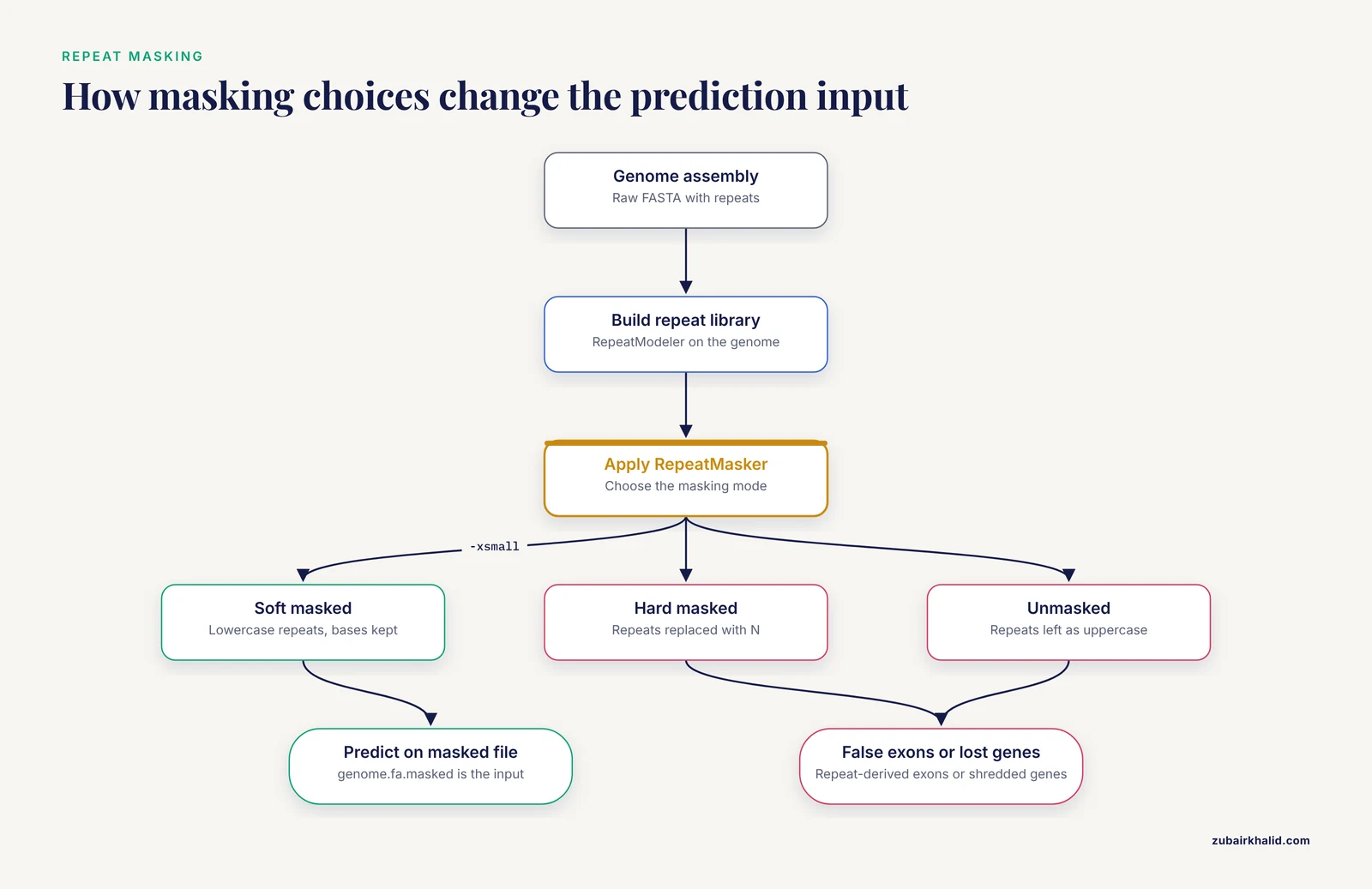
Eukaryotic predictors need to know which sequence is repetitive without destroying it. Soft masking lowercase repeats while keeping the bases, so the model can still use them in context. The standard two-tool workflow is RepeatModeler to build a species-specific repeat library, then RepeatMasker to apply it.
BuildDatabase -name genome genome.fa
RepeatModeler -database genome -pa 16 > repeatmodeler.log
RepeatMasker -pa 16 -xsmall -lib consensi.fa.classified genome.fa
The -xsmall flag tells RepeatMasker to produce soft masking. Output files are genome.fa.masked (your prediction input) and genome.fa.out (the repeat inventory, useful later).
Step 4: Baseline quality check with BUSCO
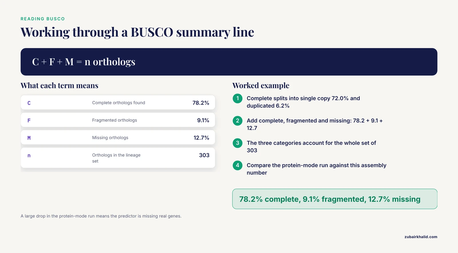
BUSCO measures assembly and annotation completeness against a set of single-copy orthologs expected in your lineage. Run it on the raw assembly so you know your ceiling before predicting genes.
busco -i genome.fa -m genome -l eukaryota -c 16 --out busco_rawThe summary in busco_raw/short_summary...txt reads like:
C:78.2%[S:72.0%,D:6.2%],F:9.1%,M:12.7%,n:303Read this as 78.2 percent of expected orthologs found as complete genes, 9.1 percent fragmented, 12.7 percent missing. If completeness is low here, gene prediction will not rescue the assembly, and you should consider reassembly first.
Step 5: A zero-evidence baseline with GeneMark-ES
Run the self-training ab initio predictor to establish a floor for your annotation.
gmes_petap.pl --ES --soft-masked --cores 16 --sequence genome.fa.masked-ES invokes the unsupervised self-training mode where parameters are estimated iteratively from the genome itself [3]. -soft-masked tells the program to interpret lowercase as repeat-masked. The main output is out.gff3 plus a log that reports the number of predicted genes and average exon statistics. Expect this run to take minutes on a fungal genome and hours on a large plant genome.
Step 6: Evidence-integrated prediction with BRAKER3
Provide homologous proteins so the pipeline can use them as hints. Any well-annotated relative's proteome works, for example the closest species in UniProt.
braker.pl --genome=genome.fa.masked \
          --prot_seq=related_proteins.fa \
          --busco_lineage=embryophyta \
          --workingdir=braker3_out \
          --threads 16
Key parameters:
-genomepoints to the soft-masked assembly.-prot_seqsupplies proteins that BRAKER aligns to the genome to generate splice-site and start/stop hints, the same hint principle that GeneMark-EP formalizes with ProtHint [4].-busco_lineagetriggers BUSCO-based training mode when no protein file is given. With proteins supplied, BRAKER uses them directly.-workingdirmust point to a directory that does not already exist, since BRAKER creates it and refuses to overwrite.
The primary output is braker.gff3 containing the final gene models, plus predicted protein and CDS FASTA files. A successful run ends with a log line reporting the number of genes predicted by the final step.
Step 7: Deep learning prediction with Helixer
Helixer runs from sequence alone using pretrained network weights, which makes it a strong independent second opinion.
Helixer.py --fasta-path genome.fa --lineage land_plantPick -lineage from the pretrained categories: vertebrate, invertebrate, land_plant, or fungi. The tool writes a GFF3 annotation plus intermediate HDF5 files. Expect substantial RAM use on large genomes because the network processes the genome in fixed-size batch windows, and note that Helixer is open source, installable locally, and also available through a web interface and Galaxy for machines without GPUs [6].
Step 8: Validate the gene models
Three checks, in increasing order of effort.
First, completeness. Run BUSCO in protein mode on the predicted proteome:
busco -i braker3_out/braker.aa -m proteins -l embryophyta -c 16 --out busco_proteinsCompleteness here should be close to the assembly-level BUSCO number from Step 4. A large drop means the predictor is missing real genes.
Second, transcript support. Align RNA-seq reads with a splice-aware aligner and check what fraction of introns are confirmed:
minimap2 -ax splice -t 16 genome.fa reads_1.fq reads_2.fq | \
    samtools sort -o aligned.bam
Third, structural plausibility. Translate predicted CDSs and look for internal stops and frameshifts, which flag false exon boundaries. This matters more than most annotators assume. An alignment-based assessment of gene structures across 47 plant genomes found that roughly 50 to 60 percent of annotated gene structures likely contained some defect, with a majority of the fixable cases recoverable by refinement against homologous consensus structures [10]. Structural errors are the norm in first-pass annotations, not the exception.
Parameter Reference
The flags below are the ones that change results most. Everything else can usually stay at defaults for a first run.
| Parameter | Tool | What it controls | When to change it |
|---|---|---|---|
-soft-masked | GeneMark | Treats lowercase bases as repeats | Always, when your input is soft-masked |
-prot_seq | BRAKER3 | Protein FASTA used for hint generation | Include whenever a related proteome exists |
-busco_lineage | BRAKER3 | BUSCO lineage for training and filtering | Match your organism's clade exactly |
-lineage | Helixer | Pretrained network selection | Must match clade, wrong lineage degrades accuracy |
-species | AUGUSTUS | Parameter set for the HMM | Use closest available trained species |
-workingdir | BRAKER3 | Output directory | Must not pre-exist |
-c / -threads | BUSCO, BRAKER3 | CPU allocation | Match available cores |
Eukaryotic Gene Prediction Tools Tips
Run the soft-masked genome for prediction, the hard-masked genome only for repeat statistics. Hard masking replaces repeats with N, which shreds any gene that contains an embedded repetitive exon. Soft masking preserves the sequence and simply tells the model where it is.
Invest in your protein set. The quality of protein hints depends on evolutionary distance. Proteins from a congeneric species outperform a broad UniProt slice, and GeneMark-EP+ showed that protein hint integration delivers its most pronounced gains in large genomes [4], where ab initio signals are weakest.
Run two independent predictors and compare, do not average. When GeneMark-EP+ and Helixer agree on a model, your confidence can be high. Where they disagree, that locus needs transcript evidence before you call it done. Reconciliation with tools like EvidenceModeler or Mikado is standard practice in production pipelines [5], and simply taking the intersection or union by hand is a reasonable start for smaller projects.
Treat full-length transcript data as the gold standard for validation. PacBio SMRT cDNA sequencing produces reads long enough to span entire transcripts, and in the sugar beet and spinach study 98 percent of full-insert SMRT reads covered complete open reading frames, which made automated gene model validation and training refinement possible for non-model genomes [11]. If your project can afford a transcriptome sequencing arm, even a small one, the gain in annotation reliability is larger than any predictor swap.
Match BUSCO lineages precisely. Running the vertebrate dataset on an insect assembly produces meaningless completeness numbers, and downstream BRAKER training inherits that error.
Log everything. Save the exact command lines, tool versions, and the GeneMark and AUGUSTUS parameter files. Reproducibility in annotation is as much about the configuration as the code, a lesson the workflow-engine platforms built for this task encode directly [5].
Keep the scope of each tool clear. If your downstream question is phylogenetic, such as reconstructing gene family trees, the gene prediction step feeds orthology inference and ultimately tree construction, and the choice of reconstruction method is its own decision with its own tradeoffs [12]. Do not try to optimize tree quality through the gene caller alone.
Common Mistakes and Limitations
Predicting on an unmasked or hard-masked genome. Both directions fail. Unmasked input floods the HMM with repeat-derived false exons. Hard-masked input deletes real coding sequence inside repeat-rich genes. Soft masking is the correct treatment, and forgetting it is the single most common first-run error.
Assuming a high-quality genome gives high-quality gene models automatically. The G3PO benchmark, built on carefully curated genes from 147 organisms, showed that ab initio gene structure prediction remains a challenging task even for well-behaved assemblies, with each program showing distinct strengths and weaknesses by gene complexity and protein length [1]. Benchmark reality is humbler than marketing.
Reusing parameters from a distant species. AUGUSTUS parameter sets trained on human degrade badly on a nematode. If your species is not pre-trained, either use a self-training tool (GeneMark-ES, Helixer) or train AUGUSTUS/SNAP on a gene set derived from your own transcript evidence.
Trusting exon boundary coordinates to the single base. First-pass models carry structural defects at high rates. The plant genome assessment found that around half to sixty percent of annotated structures likely contained defects, and that many defects traced back to pseudogenes, assembly gaps, and non-productive isoforms rather than pure algorithm failure [10]. Boundary-level refinement against homologs or transcripts is a normal second pass, not an optional luxury.
Ignoring the difference between a missing gene and a fragmented gene. BUSCO missing and fragmented categories mean different things. Fragmented models usually indicate assembly breaks or weak splice-site signals, while missing models can mean genuinely absent genes or a predictor blind spot for that gene family. Diagnose before re-running anything.
Confusing gene prediction with promoter or regulatory annotation. Promoter prediction across seven well-studied species showed that even the best computational approaches struggle with species-specific regulatory sequence recognition [9]. A complete gene model tells you where the coding region is, not how the gene is regulated.
Overreading deep learning outputs. Helixer's pretrained models are accurate and require no retraining [6], but a neural network applied far outside its training distribution can fail in ways that look superficially plausible. Cross-check at least a sample of models against homologous proteins or transcripts before committing an annotation to a repository.
Skipping the license key. GeneMark runs fail with a cryptic error when ~/.gm_key is absent. This bites nearly everyone running BRAKER for the first time.
Hardware and runtime expectations deserve a final honest note. Helixer's developers designed it to be fast and user friendly compared to resource-intensive evidence pipelines [13], yet large genomes still demand GPU or substantial CPU time, and BRAKER3 runs similarly scale with genome size. Plan compute before starting, not after the first out-of-memory failure.
Frequently Asked Questions
What are the best eukaryotic gene prediction tools?
There is no single best tool. For evidence-free annotation, GeneMark-ES and Helixer are the strongest choices, with Helixer's pretrained deep learning models matching or exceeding traditional tools across fungi, plants, vertebrates, and invertebrates [6]. For evidence-based annotation, BRAKER3 and GeneMark-EP+ are the workhorses.
Do I need RNA-seq data for gene prediction?
No. GeneMark-ES trains itself without any external data [3] and Helixer uses pretrained networks on sequence alone [6]. RNA-seq improves accuracy and validation, but a useful annotation is possible without it.
What is the difference between ab initio and evidence-based gene prediction?
Ab initio tools predict genes from sequence statistics alone using a gene structure model. Evidence-based tools add extrinsic data such as aligned proteins or RNA reads to correct and constrain predictions, which measurably improves accuracy, especially in large genomes [4].
Can I run a tool trained on one species on my new genome?
Yes, but expect reduced accuracy unless the species are close relatives. Self-training tools avoid the problem by learning from your genome directly, and deep learning tools with pretrained models generalize across clades without retraining [6].
How accurate are eukaryotic gene predictions?
Accurate enough to be useful, not accurate enough to skip validation. Independent benchmarking on 147 diverse organisms showed that ab initio gene structure prediction remains a genuinely difficult problem with tool-specific strengths and weaknesses [1], and structural defects are common enough in first-pass annotations that refinement against transcripts or homologs is standard practice [10].
How do I validate predicted gene models?
Use BUSCO completeness on the predicted proteome, align RNA-seq or long-read transcript data to confirm intron boundaries, and translate models to check for internal stop codons. Full-length PacBio SMRT reads are particularly effective for validation because nearly all full-insert reads span complete open reading frames [11].
What input files do gene prediction tools need?
The minimum is a genome assembly in FASTA format, ideally soft-masked for repeats. Evidence-based tools additionally take protein FASTA files and RNA-seq alignments in BAM format. All tools output gene coordinates in GFF3 plus predicted CDS and protein FASTA files.
How much computing power do I need?
A fungal or small insect genome annotates comfortably on a 16-core workstation. Large plant and vertebrate genomes need dozens of cores, high RAM, and ideally a GPU for Helixer. Web interfaces and Galaxy deployments exist for annotators without local high-performance computing [6].
Sources
- A benchmark study of ab initio gene prediction methods in diverse eukaryotic organisms
- An overview of computational methods for gene prediction in eukaryotes: strengths, limitations, and future directions
- Eukaryotic Gene Prediction Using GeneMark.hmm-E and GeneMark-ES
- GeneMark-EP+: eukaryotic gene prediction with self-training in the space of genes and proteins
- Long-read microbial genome assembly, gene prediction and functional annotation: a service of the MIRRI ERIC Italian node
- Helixer: ab initio prediction of primary eukaryotic gene models combining deep learning and a hidden Markov model
- Optimizing period-3 methods for eukaryotic gene prediction
- DIFFERENT GENOMIC SIGNAL PROCESSING METHODS FOR EUKARYOTIC GENE PREDICTION: A SYSTEMATIC REVIEW
- Critical assessment of computational tools for prokaryotic and eukaryotic promoter prediction
- Assessment and refinement of eukaryotic gene structure prediction with gene-structure-aware multiple protein sequence alignment
- Exploiting single-molecule transcript sequencing for eukaryotic gene prediction
- A brief overview of the concepts, methods and computational tools used in phylogenetic tree construction and gene prediction
- Helixer-de novo Prediction of Primary Eukaryotic Gene Models Combining Deep Learning and a Hidden Markov Model