How to Use Ensembl Compara for Whole-Genome Alignments
By Dr. Zubair Khalid, DVM, MS, PhD ·
By the end of this guide you will be able to open the Ensembl whole genome alignment view for any region of any Ensembl species and read it correctly, pull the same alignment blocks through the Ensembl REST API, query the public Compara MySQL server with SQL, and script larger fetches with the Perl API. You will also know which alignment method produced each track, why a region can come back empty, and how to sidestep the coordinate and assembly mistakes that cost people the most time.
On hand you need a web browser for the visual walkthrough, curl for the REST examples, and any MySQL client for the database examples. The Perl examples need Perl 5 with the Ensembl API installed. Every route shown here runs against Ensembl's public servers, so a laptop is enough compute.
Ensembl Compara is the comparative genomics arm of Ensembl, the genome database run from EMBL-EBI. Each release, Compara computes gene trees, ortholog and paralog assignments, and whole-genome alignments. A whole-genome alignment (WGA) is a precomputed alignment of complete genome assemblies against each other, stored as discrete blocks that you can view, query and download. If you are learning how to use Ensembl for comparative genomics, the browser section below doubles as a short Ensembl genome browser tutorial, and the command-line sections give you the same data in scriptable form.
What Ensembl Compara Whole-Genome Alignments Contain
Compara stores alignments under a small set of method names, and each method maps to a browser track and to a row in the method_link table you will query later. Knowing the method behind a track tells you what the blocks mean and what you can legitimately do with them.
Pairwise alignments ship under the LASTZ_NET method. LASTZ, a pairwise aligner descended from BLASTZ, aligns two genomes to each other, and a chaining and netting step then resolves overlapping hits into a hierarchy of best blocks. The net in the name refers to that hierarchy. Each block carries coordinates on both genomes, a strand, a score and a CIGAR string, which encodes the aligned and gapped positions.
Multiple alignments ship under the CACTUS method in current releases. Cactus is a progressive multiple aligner that follows the clade phylogeny and models rearrangements explicitly, and Ensembl adopted it for vertebrates in release 105 in 2021. Older releases used the EPO pipeline, with Enredo finding syntenic segments, Pecan aligning them, and Ortheus reconstructing ancestors. Those EPO tracks have been retired from recent releases, which matters because a lot of circulating tutorial material still describes them.
Two derived layers sit on top of the multiple alignments. Conservation scores store a GERP score per alignment column, where GERP measures rejected substitutions against a neutral model, so higher positive values flag positions conserved beyond expectation. Constrained elements store the intervals where those scores pass a significance threshold, which is how the browser highlights conserved noncoding segments.
New assemblies are folded into these alignments as they arrive. The 2024 naked mole-rat reference update, for example, was incorporated into multiple Ensembl whole-genome alignments as part of that release cycle [1]. Plants, metazoa, fungi and bacteria live on the separate Ensembl Genomes sites with their own Compara instances and clade-specific alignments.
One distinction saves the most confusion. Whole-genome alignments are sequence homology blocks. Orthology is a separate product built from gene trees, so a gene sitting inside an aligned block is not automatically the ortholog of your query gene. Synteny, the conservation of gene order between genomes, is a third lens again, drawn from gene-order relationships rather than base-level alignment.
| Method or track | What it is | Typical use |
|---|---|---|
| , - | , - | , - |
| LASTZ_NET | Pairwise whole-genome alignment of two genomes, chained and netted | Fine detail for one species pair, jumping between two genomes |
| CACTUS | Multiple alignment across a clade, current standard for vertebrates | Multi-species context, conservation scoring |
| EPO and EPO Extended | Legacy Enredo-Pecan-Ortheus multiple alignments of selected mammals and other clades, retired in recent releases | Reproducing older releases and publications |
| Conservation scores | GERP score per column of the multiple alignment | Quantifying conservation at individual positions |
| Constrained elements | Intervals of significant conservation from those scores | Finding conserved noncoding regions |
| Synteny | Gene-order relationships between genomes | Chromosome-scale rearrangement views |
The Ensembl Whole Genome Alignment View, Step by Step
The example uses human BRCA2, which sits on chromosome 13 at roughly 32.3 to 32.4 Mb in GRCh38, but the same clicks work for any species and region.
- Open the species and region. Go to www.ensembl.org, pick your species from the species list, and type a gene symbol such as BRCA2 or a coordinate range such as 13:32330000-32340000 into the search box. Choose the region result to land on the Region in detail view. A direct URL works too, for example
https://www.ensembl.org/Homo_sapiens/Location/View?r=13:32330000-32340000.
- Turn on the comparative tracks. Click Configure this page in the left panel and scroll to the Comparative genomics category. Switch on the Lastz Net pairwise track, the Cactus multiple-alignment track, the conservation score track and the constrained elements track. Set each to Normal and click the checkmark at the top of the panel to save. What you should see: blocks appear along the region almost immediately for a gene-sized window in a well-covered clade.
- Choose the species shown. Next to the multiple-alignment track, use the Select species option to pick which genomes display. Fewer species means a cleaner view and faster rendering. Display modes matter as well: Normal draws the full block structure, Compact collapses detail for dense regions, and Off hides the track. For a first look at a gene-sized region, Normal on both alignment tracks is the right starting point.
- Read the tracks. Pairwise blocks appear where the two genomes align, with shading that reflects block score, and the conservation track draws its score profile across the region. Empty stretches mean no net block passed the pipeline thresholds there, which is common over repeats and assembly gaps.
- Open a block. Click any alignment block. A menu opens with options such as View alignment, which opens a base-level display with the reference sequence on top, the aligned sequence below, a match line between them, and identity information for the block, plus navigation to move to the previous or next block.
- Cross species. Use the jump option in that menu to open the aligned region in the other species. The other genome opens at the aligned coordinates in the same Region in detail view, so you can walk along a syntenic chain block by block.
- Compare several species at once. Open the Compare menu at the top of the page and choose Location, then add species from the Select species panel. The view stacks the same region from several genomes with alignment blocks drawn between them. Zoom out to chromosome scale to see syntenic blocks and rearrangements.
- Cross-reference the gene view. From a gene page, the left menu under Comparative genomics lists Gene tree, Orthologues and Paralogues. Reading the gene tree next to the alignment view tells you whether the conserved sequence you see belongs to an ortholog, a paralog or a repeat.
- Verify the setup. The banner above the view names the species, assembly and release, and the track legend names the method and species set. Record both before you screenshot anything for a paper.
Fetching Alignments with the Ensembl REST API
The REST API, the HTTP interface Ensembl publishes for programmatic access, returns the same blocks the browser draws, as JSON. It is the quickest scripted route.
The endpoint is /alignment/region/:species/:region on rest.ensembl.org. The species takes the Ensembl name, homo_sapiens. The region takes seq_region:start-end in 1-based inclusive coordinates. The method parameter filters by alignment method.
curl -s -H "Content-Type:application/json" \
  "https://rest.ensembl.org/alignment/region/homo_sapiens/13:32330000-32340000?method=LASTZ_NET"
The response is a JSON array with one entry per aligned sequence per block. Fields include the species, the seq_region name, start, end, strand and a CIGAR string. Truncated illustrative output, with values that will differ on your run:
[
  {
    "species": "homo_sapiens",
    "seq_region": "13",
    "start": 32331102,
    "end": 32331897,
    "strand": 1,
    "cigar": "796M"
  },
  {
    "species": "mus_musculus",
    "seq_region": "12",
    "start": 33987401,
    "end": 33988196,
    "strand": 1,
    "cigar": "796M"
  }
]
Swap method=LASTZ_NET for method=CACTUS to pull the multiple alignment, and check the endpoint page at rest.ensembl.org for the optional parameters that restrict the species set or trim the response. Endpoint paths occasionally change between API versions, so confirm the path on the endpoint list if a call returns a 404. An empty JSON array means no blocks for that method in that region, so try the other method or widen the interval before assuming a bug.
Errors come back as JSON with an error key, usually for a malformed region string or an unrecognized species name. Ensembl applies a per-second rate limit to REST traffic, so add a short sleep between calls when scripting and batch regions where the endpoint allows it. If headers are awkward in your tooling, pass the content type as a query parameter instead.
The same API carries the homology data you will want next to the alignments. This call lists BRCA2 orthologs:
curl -s -H "Content-Type:application/json" \
  "https://rest.ensembl.org/homology/id/human/ENSG00000139618?type=orthologues"
Each hit carries the target species, the target gene or protein identifier, and the confidence labels Ensembl assigns to the relationship, which you can compare against the aligned blocks you just pulled.
Querying the Public Compara MySQL Server
Ensembl publishes the databases behind the website on a public MySQL server. The server is read-only, the user is anonymous, and no password is needed. This route is the best way to understand the schema, because the browser and the REST endpoint are thin layers over exactly these tables.
mysql -h ensembldb.ensembl.org -P 3306 -u anonymousStep 1. Find the current Compara database. Release numbers change every few months, so never hardcode one you have not confirmed.
SHOW DATABASES LIKE '%compara%';Illustrative output:
+----------------------+
| Database (%compara%) |
+----------------------+
| ensembl_compara_111  |
+----------------------+
The number matches the current release. Use whatever your server returns.
USE ensembl_compara_111;Step 2. List the alignment methods in this release.
SELECT method_link_id, type
FROM method_link
WHERE type IN ('LASTZ_NET','CACTUS','EPO','EPO_EXTENDED',
               'GERP_CONSERVATION_SCORE','GERP_CONSTRAINED_ELEMENT');
Illustrative output, with release-specific IDs:
+----------------+--------------------------+
| method_link_id | type                     |
+----------------+--------------------------+
|              2 | LASTZ_NET                |
|             12 | CACTUS                   |
|             16 | GERP_CONSERVATION_SCORE  |
|             17 | GERP_CONSTRAINED_ELEMENT |
+----------------+--------------------------+
If EPO rows are missing, your release has retired them. The type strings are what matter, not the IDs.
Step 3. Confirm the genomes and assemblies. The genome_db table lists the genomes, and dnafrag rows are the individual sequences within each genome.
SELECT name, assembly FROM genome_db
WHERE name IN ('homo_sapiens','

## Finishing the MySQL Walkthrough: Joins That Turn Tables into Alignments

The Compara schema looks intimidating at first, but it follows one clean idea: every alignment block is stored once, and every genome's view of that block is stored as a separate row that points back to it. Once that clicks, the queries write themselves.

The central pair of tables works like this. `genomic_align_block` holds one row per alignment block, tagged with the `method_link_species_set_id` that identifies which alignment method and species set produced it. `genomic_align` holds one row per genome per block, tagged with the same block identifier, and carries that genome's coordinates on its own `dnafrag`, its strand, and its CIGAR string. `dnafrag` is one sequence, usually one chromosome, within a genome, and it points to `genome_db`, which names the genome and its assembly. `method_link_species_set` ties a method from `method_link` to a species set, and its human readable `name` column is the label you see in the browser track legend.

Before writing any join, list the available pairwise alignments by name, because the name string is the fastest way to pick the right `method_link_species_set_id`:
SELECT mlss.method_link_species_set_id, mlss.name FROM method_link_species_set mlss JOIN method_link ml ON ml.method_link_id = mlss.method_link_id WHERE ml.type = 'LASTZ_NET' AND mlss.name LIKE '%Human%Mouse%';
Illustrative output, with release specific identifiers:
+--------------+-------------+
| method_link_species_set_id | name |
|---|
+--------------+-------------+
| 269 | LASTZ_NET Human vs Mouse |
|---|
+--------------+-------------+
Store that identifier in a session variable so your main query stays readable, then pull every block that overlaps your region and, for each block, every other genome's view of the same block:
SET @mlss = 269; SET @hchr = '13'; SET @hstart = 32330000; SET @hend = 32340000;
SELECT g2.name AS species, df2.name AS chromosome, ga2.dnafrag_start AS aln_start, ga2.dnafrag_end AS aln_end, ga2.dnafrag_strand AS strand, ga2.cigar_line AS cigar FROM genomic_align ga1 JOIN dnafrag df1 ON df1.dnafrag_id = ga1.dnafrag_id JOIN genome_db g1 ON g1.genome_db_id = df1.genome_db_id JOIN genomic_align_block gab ON gab.genomic_align_block_id = ga1.genomic_align_block_id JOIN genomic_align ga2 ON ga2.genomic_align_block_id = ga1.genomic_align_block_id JOIN dnafrag df2 ON df2.dnafrag_id = ga2.dnafrag_id JOIN genome_db g2 ON g2.genome_db_id = df2.genome_db_id WHERE gab.method_link_species_set_id = @mlss AND g1.name = 'homo_sapiens' AND df1.name = @hchr AND ga1.dnafrag_start <= @hend AND ga1.dnafrag_end >= @hstart AND g2.name <> 'homo_sapiens' ORDER BY ga1.dnafrag_start, g2.name, ga2.dnafrag_start;
Read the query from the inside out. The filters on `ga1` select the human side of every block touching your window. The join through `genomic_align_block` finds the blocks themselves, and the second join onto `genomic_align ga2` finds the partner rows, one for each other genome in the alignment. The final joins resolve those partner rows into species and chromosome names you can actually read.

Three practical cautions for these tables:

1. **Always filter on the method link species set first.** The `genomic_align` tables are among the largest in Compara. A query that scans without the `method_link_species_set_id` predicate can take minutes; with it, the server uses the indexes and answers in seconds.
2. **Restrict on the `dnafrag` before filtering coordinates.** Filtering by chromosome name first, then by coordinate overlap, keeps the working set small.
3. **Run `DESCRIBE` before you commit to a join.** Table columns shift slightly between releases. `DESCRIBE genomic_align;` and `DESCRIBE conservation_score;` take two seconds and save a broken script later. This habit also covers you when a release rebuilds the database from scratch, which happens every cycle as new assemblies are folded into the alignments [1].

Exporting the result for downstream tools takes one more flag set. Batch mode gives tab separated rows with no table furniture:
mysql -h ensembldb.ensembl.org -P 3306 -u anonymous -N -B -e \ "USE ensembl_compara_111; SELECT g2.name, df2.name, ga2.dnafrag_start, \ ga2.dnafrag_end, ga2.dnafrag_strand, ga2.cigar_line \ FROM genomic_align ga1 \ JOIN genomic_align_block gab ON gab.genomic_align_block_id = ga1.genomic_align_block_id \ JOIN genomic_align ga2 ON ga2.genomic_align_block_id = ga1.genomic_align_block_id \ JOIN dnafrag df2 ON df2.dnafrag_id = ga2.dnafrag_id \ JOIN genome_db g2 ON g2.genome_db_id = df2.genome_db_id \ JOIN dnafrag df1 ON df1.dnafrag_id = ga1.dnafrag_id \ WHERE gab.method_link_species_set_id = 269 \ AND df1.name = '13' \ AND ga1.dnafrag_start <= 32340000 \ AND ga1.dnafrag_end >= 32330000 \ AND df1.genome_db_id = (SELECT genome_db_id FROM genome_db WHERE name = 'homo_sapiens') \ AND g2.name <> 'homo_sapiens';" > mouse_blocks.tsv
The output has six columns: species, chromosome, start, end, strand, CIGAR. One subtlety worth knowing now: Ensembl stores coordinates with start always less than or equal to end, even on the reverse strand. The strand column, not the coordinate order, tells you the orientation. Code that assumes start greater than end means minus strand will silently misbehave.

## Worked Example: Mapping a Human Gene onto the Mouse Genome End to End

Here is the full pipeline for a realistic task: you have the human BRCA2 locus and you want every mouse block that aligns to it, exported as BED for downstream work.

**Step 1. Pull the blocks from REST.**
curl -s -H "Content-Type:application/json" \ "https://rest.ensembl.org/alignment/region/homo_sapiens/13:32330000-32340000?method=LASTZ_NET" \
brca2_lastz.json
**Step 2. Extract the mouse side as BED.** BED uses zero based, half open coordinates, while the REST response uses one based, inclusive coordinates, so subtract one from every start:
jq -r '.[] | select(.species=="mus_musculus") | [.seq_region, .start-1, .end, .cigar] | @tsv' brca2_lastz.json > mouse_blocks.bed4
**Step 3. Expand the CIGAR to count aligned bases.** The `start` and `end` in the response span the block including its internal gaps, so a block with a large deletion looks longer on the target genome than its matched base count justifies. Count the M tokens when the aligned base count matters:
perl -ne 'chomp; my @f = split /\t/; my $m = 0; while ($f =~ /(\d+)([MID])/g) { $m += $1 if $2 eq "M"; } print join("\t", @f, $m), "\n";' mouse_blocks.bed4 > mouse_blocks.bed5
The fifth column is now the number of alignment columns where both genomes contribute a base. Keep in mind that M in Ensembl Compara CIGAR strings includes mismatches, so this count is aligned columns, not identities. If you need identities, open the block in the browser alignment view, which reports identity per block, or align the extracted sequences yourself with a dedicated tool.

**Step 4. Sort and inspect.**
sort -k1,1 -k2,2n mouse_blocks.bed5 | column -t | head
**Step 5. Sanity check against the browser.** Open the same region in the Ensembl whole genome alignment view with the Lastz Net track on and count the mouse blocks drawn. You should get the same number of blocks as rows in your file. If the counts differ, the most common cause is a filter: the browser view and the REST call must use the same method, and the browser may be showing species you filtered out in `jq`.

**Step 6. Cross reference orthology.** Alignment says the sequence is homologous; the gene tree says the gene is orthologous. Pull the mouse ortholog for BRCA2 and check whether its coordinates fall inside one of your blocks:
curl -s -H "Content-Type:application/json" \ "https://rest.ensembl.org/homology/id/human/ENSG00000139618?type=orthologues" \ | jq -r '.data[].homologies[] | select(.target_species=="mus_mouse") | .target.id'
Note two things about this call. The species token in the homology endpoint uses the display style Ensembl uses for homology responses, so if the filter above returns nothing, drop the `select` and inspect the raw JSON to see the exact species strings before filtering. And the confidence labels in the response matter: an ortholog with a weaker confidence annotation that sits outside your aligned blocks is telling you something worth investigating, not necessarily a bug in your pipeline.

**Step 7. Record provenance.** Write the release number, the method string, the exact region, the assembly of both genomes, and the date into a small manifest file beside your outputs. Six months from now, this manifest is the only thing standing between your results and an unreproducible mystery, especially since each release can fold updated assemblies into the alignments [1].

## Scripting Larger Fetches with the Ensembl Perl API

The Perl API is the right tool when a task outgrows one off queries: iterating over hundreds of genes, computing per block statistics, or walking chains of blocks across a chromosome. It gives you objects rather than JSON or rows, which removes all coordinate and CIGAR parsing from your code.

**Installation and connection.** Install the Ensembl core and Compara API checkouts per the instructions on the Ensembl API documentation pages, and keep both at the same release. The registry loader connects to the public server exactly like the MySQL client does:
#!/usr/bin/perl use strict; use warnings;
use Bio::EnsEMBL::Registry; use Bio::EnsEMBL::Compara::DBSQL::DBAdaptor;
Core API: resolve slices against the matching release
Bio::EnsEMBL::Registry->load_registry_from_db( -host => 'ensembldb.ensembl.org', -user => 'anonymous', -port => 3306, );
Compara API: attach the release matched Compara database
my $compara = Bio::EnsEMBL::Compara::DBSQL::DBAdaptor->new( -host => 'ensembldb.ensembl.org', -user => 'anonymous', -port => 3306, -dbname => 'ensembl_compara_111', );
The release number in the database name must match the release your registry loaded. Mismatches surface as confusing errors about missing species or methods, and they are the single most common Perl API failure on the public server.

**Fetch the alignment objects.**
my $mlss_adaptor = $compara->get_MethodLinkSpeciesSetAdaptor(); my $mlss = $mlss_adaptor->fetch_by_method_link_type_GenomeDBs( 'LASTZ_NET', $compara->get_GenomeDBAdaptor()->fetch_by_name_assembly('homo_sapiens'), $compara->get_GenomeDBAdaptor()->fetch_by_name_assembly('mus_musculus'), );
my $slice_adaptor = Bio::EnsEMBL::Registry->get_adaptor( 'homo_sapiens', 'core', 'Slice'); my $slice = $slice_adaptor->fetch_by_region( 'chromosome', '13', 32330000, 32340000);
my $gab_adaptor = $compara->get_GenomicAlignBlockAdaptor(); my $blocks = $gab_adaptor->fetch_all_by_MethodLinkSpeciesSet_Slice( $mlss, $slice);
**Iterate and report.** Each `GenomicAlignBlock` holds a list of `GenomicAlign` objects, one per genome, each carrying a `dnafrag`, coordinates, a strand and a CIGAR line:
foreach my $block (@$blocks) { foreach my $ga (@{ $block->get_all_GenomicAligns() }) { printf "%s\t%s\t%d\t%d\t%d\t%s\n", $ga->genome_db->name, $ga->dnafrag->name, $ga->dnafrag_start, $ga->dnafrag_end, $ga->dnafrag_strand, $ga->cigar_line; } }
This prints the same six fields as the MySQL query above, obtained through objects that enforce coordinate conventions for you.
**Practical advice for larger runs.**
- Wrap the fetch loop in progress logging with block counts per region, because silent partial failures are hard to spot in long runs.
- Batch by gene or by fixed megabase windows rather than fetching a whole chromosome at once. Whole chromosome fetches of pairwise nets are heavy for both your memory and the shared server.
- Add a polite delay between regions even though the Perl API does not enforce the REST style per second limit; you share the public server with everyone else.
- Keep a single configuration file with the release number and database name, and require every script to read it. When release 112 replaces 111, you change one line.
- Test each new script against a tiny region first, ideally one you have already validated in the browser, so you know the code rather than the data is at fault when output looks wrong.
The Perl API also exposes the derived layers: adaptors exist for the conservation and constrained element results, and the object model mirrors the schema you explored in SQL. If you find yourself writing a third SQL query for the same analysis, it is usually time to move that logic into Perl or Python against the API.
## Conservation Scores and Constrained Elements in Practice
The derived layers deserve their own treatment because they answer a different question than the alignment tracks. Alignments tell you where sequence is homologous. Conservation scores and constrained elements tell you where homologous sequence is evolving more slowly than a neutral model predicts, which is the signal people usually want when hunting for functional noncoding regions.
**Reading GERP values correctly.** The conservation score track plots a GERP score per alignment column. Positive values indicate rejected substitutions, meaning the position has conserved more than expected under neutrality, and the value scales with the strength of that excess. Near zero means the position evolves neutrally. The score depends on the alignment and the species set behind it, so a score from a 100 mammal alignment is not directly comparable to one from a narrower panel. When you quote a score in a report, quote the method and species set with it.
**Finding constrained elements for your region.** In the browser, switch on the constrained elements track alongside the conservation score track. The elements are the intervals where the per column scores jointly pass a significance threshold, and they are the practical units for annotation: a variant inside a constrained element in an otherwise unconstrained locus is a much stronger candidate than the same variant in unconstrained aligned sequence.
**Querying the scores in SQL.** The `conservation_score` and `constrained_element` tables store these results, keyed to their own method link species sets, which you find with the same query pattern as before, filtering `method_link` on the GERP types. Because column layouts for these tables vary between releases, make `DESCRIBE conservation_score;` the first statement of any session that touches them, then write your join against what the release actually provides. Typical queries select score rows overlapping your region and join to the constrained element identifier so you can report per element aggregates such as mean score.
**A concrete interpretation routine.** For a candidate regulatory variant:
1. Open the region in the browser with the conservation score and constrained element tracks on.
2. Note whether the variant falls inside a constrained element and, if so, which clade the element was called in.
3. Read the local score profile. A variant on a broad conservation plateau reads differently from one on a narrow peak, and both differ from a variant in unconstrained sequence.
4. Check the alignment view for the same column. A high score over a column that only aligns two distantly related genomes deserves more skepticism than the same score in a densely aligned mammalian block.
5. Pull the exact per column scores from SQL if you need to report them numerically, with the release and method recorded.
**One trap to avoid.** Absence of a constrained element is not evidence of absence of function. Elements are called against a statistical model with thresholds, alignment errors suppress scores, and regions absent from the multiple alignment entirely carry no scores at all. Report constrained elements as one line of evidence among several, never as a verdict.
## Ensembl Whole Genome Alignment View Tips: Reading Tracks Correctly
The visual view encodes a lot of information in small graphical choices, and a few reading habits will make you much faster.
**Understand the net structure before interpreting block shading.** LASTZ_NET blocks are not flat. The netting step organizes overlapping alignment hits into a hierarchy where the best scoring chain occupies the primary level and displaced or overlapping hits appear as nested descendants. Visually this can look like several blocks of different shading stacked over one locus. That is not redundancy: the hierarchy is telling you which alignment the pipeline ranked first and which alternatives it displaced. If you export blocks programmatically, decide explicitly whether you want the whole net or only top level blocks, because a naive export mixes levels.
**Match display mode to question.** Normal mode draws full block structure and is right for reading a gene sized interval. Compact mode trades detail for density and is right for scanning a chromosome arm. At very wide zoom levels the browser aggregates blocks, and individual block boundaries may not be resolvable, so never make block level claims from a chromosome scale screenshot; zoom in and confirm.
**Use the identity information, not block width, as your quality cue.** Two blocks of identical width can differ enormously in match fraction. The alignment popup reports identity for the block, and that number, not length, is what you should cite when justifying a conserved segment claim.
**Check strand when comparing orientation.** A block on the reverse strand in the partner genome is visually obvious in the pairwise view, but when you export coordinates to BED and later intersect them with features, a missed strand flips your interpretation. Make strand part of every exported record.
**Treat empty stretches as information.** A gap in the alignment track over a repeat rich stretch usually means no net block passed thresholds there. Over a poorly assembled region it means the partner genome's sequence is genuinely missing or fragmented. The two cases look identical on the track, so check the partner genome's assembly status before concluding a region is nonconserved.
**Pair the alignment view with the gene tree view.** The single most informative habit in comparative browsing is opening the gene tree for the gene in your region next to the alignment tracks. Sequence conservation inside an intron between species whose genes are paralogs tells a very different story from the same pattern between orthologs.
**Screenshot with context.** Before any figure for a paper or thesis, capture the banner showing species, assembly and release, and the track legend naming the method. Reviewers increasingly ask, and your future self certainly will.
## Ensembl Whole Genome Alignment View Common Mistakes
These are the errors that cost the most time, listed with the symptom each one produces and the fix.
**Mistake 1: Treating an alignment block as an ortholog.** The block says the sequence is homologous. Orthology is assigned from gene trees in a separate product. A duplicated gene can sit inside an aligned block next to a paralog of your query gene. Fix: always cross check the gene tree or the homology endpoint before calling a gene in a block an ortholog.
**Mistake 2: Mixing assemblies.** Coordinates are assembly specific. A region from GRCh37 will not land where you expect in a GRCh38 view, and mouse coordinates from GRCm38 versus GRCm39 differ as well. Symptom: your exported region looks empty or shifted. Fix: confirm the assembly in the banner for both the query and partner genomes, and re query under the correct assembly.
**Mistake 3: Assuming EPO era tutorials still work.** A large amount of circulating material describes the Enredo, Pecan and Ortheus pipeline and its track names. Recent releases retired those tracks in favor of Cactus. Symptom: a tutorial track name does not exist in the configure panel. Fix: use the Cactus track for multiple alignment and check the current method list in the `method_link` table.
**Mistake 4: Ignoring coordinate system boundaries.** The REST endpoint takes one based inclusive coordinates. BED takes zero based half open intervals. Ensembl chromosome names lack the `chr` prefix that UCSC tools expect. Symptom: off by one shifts after export, or BED tools that find nothing. Fix: convert deliberately, once, in one documented place in your pipeline, and normalize chromosome names on export.
**Mistake 5: Reading CIGAR M as identity.** M tokens cover aligned columns including mismatches. Symptom: inflated conservation estimates. Fix: count mismatches explicitly if you need identity, or read the per block identity in the browser.
**Mistake 6: Exporting the whole net when you wanted the top level.** Symptom: duplicated or nested coverage over one locus in downstream intersection. Fix: filter to top level blocks if that is your intent, and record which choice you made.
**Mistake 7: Querying the wrong release.** Hardcoded database names like `ensembl_compara_111` break when the server rolls over. Symptom: `Unknown database` errors. Fix: discover the current name with `SHOW DATABASES LIKE '%compara%';` inside the script.
**Mistake 8: Assuming the species you want is in the alignment.** Every alignment covers a defined species set. If your species is not in it, every query is legitimately empty. Symptom: empty arrays and empty tracks for one species while others work. Fix: check the species set behind the method link species set before debugging anything else.
**Mistake 9: Forgetting that assemblies get updated.** A reference you analyzed last year may itself have been superseded, and the new assembly enters the whole genome alignments as part of the release cycle [1]. Symptom: results that differ subtly between two runs months apart with identical code. Fix: pin a release for the whole project and record it.
**Mistake 10: Confusing the synteny view with the alignment view.** Synteny derives from gene order relationships, not base level alignment. A syntenic block can contain unaligned sequence and vice versa. Fix: use the synteny view for chromosome scale rearrangement questions and the alignment view for sequence level questions, and say which one your claims come from.
**Mistake 11: Looking for clade alignments in the wrong place.** Plants, metazoa, fungi and bacteria live on the Ensembl Genomes sites with their own Compara instances. Symptom: your plant species has no tracks on the main site. Fix: switch to the relevant Ensembl Genomes portal for nonvertebrate clades.
## Troubleshooting Empty Tracks, Failed Calls and Broken Scripts
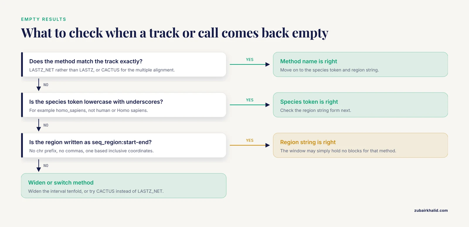
Work down this list whenever a step in the guide misbehaves. The ordering runs from most to least common.
**Empty REST response but the browser shows blocks.** Check three things in order: the method parameter matches the track exactly, for example `LASTZ_NET` rather than `LASTZ`; the species token is the Ensembl name in lowercase with underscores; and the region string uses the `seq_region:start-end` form with no chromosome prefix or commas. If all three look right, widen the interval by a factor of ten; a one kilobase window in a sparse region is often legitimately empty.
**404 from REST.** Endpoint paths occasionally change between API versions. Confirm the path on the endpoint list at rest.ensembl.org, and check that you are calling the stable root rather than a versioned path unless you intended to.
**Rate limit responses during a loop.** Ensembl applies a per second limit to REST traffic. Add a sleep of a fraction of a second between calls, batch regions where the endpoint supports it, and retry with backoff on throttling responses rather than hammering.
**`Unknown database` in MySQL.** The release suffix rolled over. Run `SHOW DATABASES LIKE '%compara%';` and use what it returns. Any script with a hardcoded suffix will eventually break this way, including perfectly working ones from last quarter.
**`Unknown column` or strange rows in SQL.** Schema drift between releases. Run `DESCRIBE` on each table you join and rebuild the query against the current layout rather than a remembered one.
**Impossibly slow SQL.** Almost always a missing `method_link_species_set_id` or `dnafrag` filter. Restrict first on method and chromosome, then apply coordinate filters.
**Browser tracks present but blank.** The display mode is probably set to Off, or the species you expect is not selected in the Select species panel for that track. Reopen the configure panel and confirm both.
**Perl API errors about missing species or mismatched versions.** The Compara database name and the registry release disagree. Align both to the same release number, and verify with a trivial fetch of one known slice before running the real script.
**Blocks that vanished between two runs.** You are probably hitting different releases. The database is rebuilt each cycle, and updated assemblies enter the alignments as part of that cycle [1]. Check the release banner or the database suffix, then either pin the old release via the archive site or accept and document the new one.
**Results that differ from a published table.** Before suspecting your pipeline, check the paper's release year. A 2019 figure built on the EPO pipelines cannot be reproduced against a current Cactus based release. Reproduce historical results on the matching archived release instead.
## Choosing Between the Browser, REST, MySQL, Perl and Bulk Files
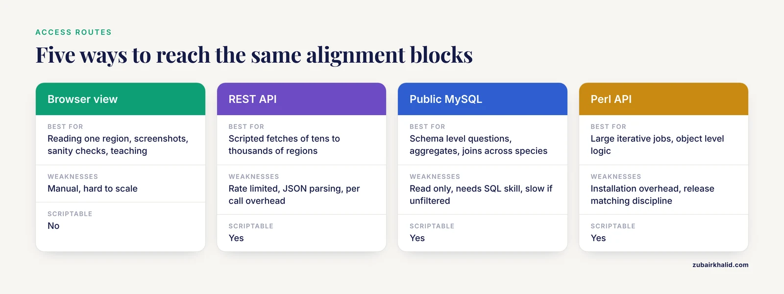
Each access route has a sweet spot, and picking the right one up front saves hours.
| Route | Best for | Weaknesses |
| -- | -- | -- |
| Browser view | Reading one region, screenshots, sanity checks, teaching | Not scriptable, manual, hard to scale |
| REST API | Scripted fetches of tens to thousands of regions, quick prototyping | Rate limited, JSON parsing, per call overhead |
| Public MySQL | Schema level questions, aggregates, joins across methods and species | Read only, requires SQL skill, slow if unfiltered |
| Perl API | Large iterative jobs, object level logic, integrating with Ensembl core objects | Installation overhead, release matching discipline |
| Bulk files | Very large or repeated analyses, MAF style whole alignment downloads | Big downloads, less current than per release pinning, parsing effort |
A reasonable workflow for most projects looks like this: explore the region in the browser to learn what is there; prototype the extraction in REST for one or two regions; move to the Perl API or MySQL when the region list grows past dozens; and switch to bulk downloads only when the analysis is genome scale or will be repeated against many releases. Mixing routes is normal and fine as long as every route resolves to the same release, method and assemblies, which is why the manifest habit from the worked example matters across the whole project.
One comparison worth making explicit: the browser and REST return the same underlying blocks, so any discrepancy between them is a filter or parameter problem, not a data problem. The MySQL route can answer questions the other two cannot, such as how many blocks a given pair of genomes shares genome wide, because it exposes the full schema rather than a single region slice.
## Practical Applications of Whole-Genome Alignment Data
**Prioritizing candidate regulatory variants.** For a GWAS hit or a candidate enhancer, overlay the interval on the constrained elements track, pull the overlapping elements from SQL, and report the GERP profile. A noncoding variant inside a mammalian constrained element is a defensible priority for functional follow up, and the alignment view gives you the visual evidence for the figure.
**Cross species primer and reagent design.** Pull LASTZ_NET blocks between your species of interest and a model organism, filter blocks by size and aligned base count from the CIGAR expansion, and design primers inside blocks whose identity the browser confirms. This works well for degenerate PCR across related species and for designing probes that should bind multiple genomes.
**Sanity checking coordinate conversions.** Before trusting an automated liftover of a variant or a feature set, manually align the source region in the whole genome alignment view and confirm the lifted coordinates fall inside a block with the expected strand. Liftover tools and Compara nets do not always agree at block boundaries, and five minutes in the browser catches most disagreements.
**Building custom tracks.** The BED exports from the worked example load directly into IGV or JBrowse as custom tracks alongside your own data. A common and effective figure layers your variant calls or ChIP peaks over the Compara constrained elements for the same interval.
**Supporting orthology claims in manuscripts.** Combining the gene tree, the homology endpoint output and the sequence level alignment block in one figure is a much stronger orthology claim than any single one alone, and the three views cross validate each other.
**Teaching and training.** The browser walkthrough scales beautifully to a classroom because it needs nothing but a browser, and the BRCA2 example generalizes: pick a gene students care about, walk the eight steps, then have each student repeat it for a different species pair. The inevitable surprises, empty tracks and unexpected paralogs, are the best teaching moments in comparative genomics.
**Quality control for assemblies and annotations.** If you work with a recently updated assembly, checking that your gene of interest now sits inside expected alignment blocks against well annotated relatives is a fast structural check on the new assembly, which is exactly the kind of verification that release cycles with fresh assemblies invite [1].
## Release Management and Reproducibility for Compara Work
Compara is a moving target by design. Releases arrive every few months, methods get retired, assemblies get updated and folded into the alignments [1], and database names change suffixes. None of that is a problem if you manage it deliberately.
**Pin a release per project.** Choose the release at project start, record it in your manifest and configuration files, and use the archive site if you must return to it later. Every number you publish should be traceable to one release.
**Record the full identification tuple.** For every result, log the release, the method string, the method link species set identifier, both assemblies, the exact coordinates, and the access route. A result described only as "from Ensembl Compara" is not reproducible; one described as "release 111, LASTZ_NET Human versus Mouse, MLSS 269, GRCh38 region 13:32330000 to 32340000" is.
**Archive raw responses.** Save the JSON from every REST call and the TSV from every SQL export before post processing. Re running a query months later can return different data after a release rollover, so the raw capture is your only stable evidence.
**Plan for the next release.** Put a release check at the top of every script: query the current database name, compare it with the manifest, and either warn or abort on mismatch. This turns a silent reproducibility failure into a loud, actionable error.
**Write methods sections as you go.** The banner, legend and manifest details you collect for screenshots are also the raw material for your methods paragraph. Draft it during the analysis rather than at submission time, when the release has likely moved on and memory is unreliable.
Handled this way, the moving release cycle becomes an advantage rather than a hazard: your work inherits each improvement in assemblies and alignments automatically, and you always know exactly which version of the data any given result rests on.
## Further Reading
- [Conceptual framework and pilot study to benchmark phylogenomic databases based on reference gene trees.](https://pubmed.ncbi.nlm.nih.gov/21737420/)
## Sources
1. [An updated reference genome sequence and annotation reveals gene losses and gains underlying naked mole-rat biology.](https://pubmed.ncbi.nlm.nih.gov/39651266/)