Ensembl Region in Detail View
By Dr. Zubair Khalid, DVM, MS, PhD ·
The Ensembl Region in Detail view is the main coordinate-based display of the Ensembl genome browser, showing a chosen stretch of a chromosome as horizontal tracks filled with genes, transcripts, variants, regulatory features, and comparative data. It sits in the middle of the Location page, between the chromosome-wide Region overview above it and the basepair-level sequence view that appears when you zoom in far enough.
Most questions in genomics are regional questions. A clinical laboratory reports a deletion at 17q21.31, a genome-wide association study flags a signal on chromosome 7, or an RNA-seq experiment turns up an unannotated isoform, and the first move is always the same: open that exact stretch of the reference genome and see what is annotated there. Region in Detail renders the contents of the Ensembl databases as a picture you can read at a glance [1]. It also accepts your own data as extra tracks, which is why clinical interpretation platforms such as DECIPHER build their region-navigation workflow on the Ensembl browser [2] and why custom plug-ins such as Statistical Viewer extend it with study-specific plots [3]. If you learn one Ensembl panel well, learn this one. The sections below explain the view from the database up, walk through it as a hands-on Ensembl genome browser tutorial, and then interpret its tracks one by one.
What the Region in Detail View Means
The word region refers to a span of coordinates on a reference assembly, not to a gene and not to a picture of anyone's personal genome. Each species has its own assembly and therefore its own coordinate space. For human, the current reference is GRCh38, and a region is written chromosome:start-end, for example 17:43044295-43125482. The same biological position on the previous human reference, GRCh37, carries different coordinates, which is why assembly labels matter so much.
The word detail is relative. The Location page is a zoom hierarchy with three levels:
- Region overview. The full chromosome drawn as an ideogram, a schematic chromosome map with cytogenetic bands, and a red box marking the window you are viewing.
- Region in detail. The selected window drawn as parallel tracks of annotated features. The on-screen label reads Region in detail.
- Basepair view. Once the window narrows below a browser-defined threshold, a sequence panel appears at the bottom, showing actual nucleotides with a six-frame translation.
The panels stay synchronized. Click a band in the ideogram and the detail view jumps there. Click a feature in the detail view and its report page opens. Zoom, and all three levels update together.
A note on names saves confusion when you read older literature. Ensembl releases before the interface redesign called the detailed view ContigView and the chromosome view CytoView, and papers from that era use those labels, as in the Statistical Viewer description of panels drawn on Contig View and Cyto View pages [3]. Region in Detail is the modern successor to ContigView, with the same core idea: one coordinate window, many annotation tracks.
Just as useful is knowing what the view is not. It is not a report about one gene, which is what the gene report pages provide. It is not a read-alignment viewer for your own sequencing files, although track hubs can display such data. It is not an analysis environment, because the picture cannot compute anything. Treat it as a coordinate-anchored summary of everything the Ensembl databases know about a span of DNA, and treat every number you actually care about as something to export and measure.
Terms It Gets Confused With
| View or term | What it shows | Typical use | Relationship to Region in Detail |
|---|---|---|---|
| Region overview | The whole chromosome as a banded ideogram with a red box around your window | Orienting yourself before zooming | Parent panel, sits directly above |
| Region in Detail | Annotated tracks for the selected coordinate window | Reading genes, variants, and regulation in context | The main working view |
| Basepair view | Nucleotide sequence with six-frame translation at high zoom | Codon checks, primer design | Child panel, appears at high zoom |
| Location tab | The browser page containing all three panels | Container and navigation hub | Region in Detail is the middle panel of this tab |
| ContigView (legacy) | The detailed view in pre-redesign Ensembl releases | Reading older papers and screenshots | Superseded by Region in Detail |
| Gene report page | A report for one gene or transcript | Deep dive on a single feature | Opened by clicking a feature inside the view |
| Track hub | A remote bundle of user or third-party tracks | Adding large datasets such as alignments | Rendered as extra tracks inside the view |
| REST API, BioMart | Programmatic access to the same underlying data | Pipelines and bulk analysis | Same data as the view, without the picture |
How the Browser Builds the View
Four pieces of machinery produce everything you see, and knowing them makes the view easier to interpret and easier to troubleshoot.
The core schema. Ensembl stores genome annotation in a relational schema built around four central tables: gene, transcript, exon, and translation. The Ensembl gene-building system annotates genomes automatically from evidence derived from known protein, cDNA, and expressed sequence tag (EST) sequences, and it rests on this core MySQL schema and Perl API [1]. When the view draws a gene track, it queries those tables for every model overlapping your coordinates and stacks the results.
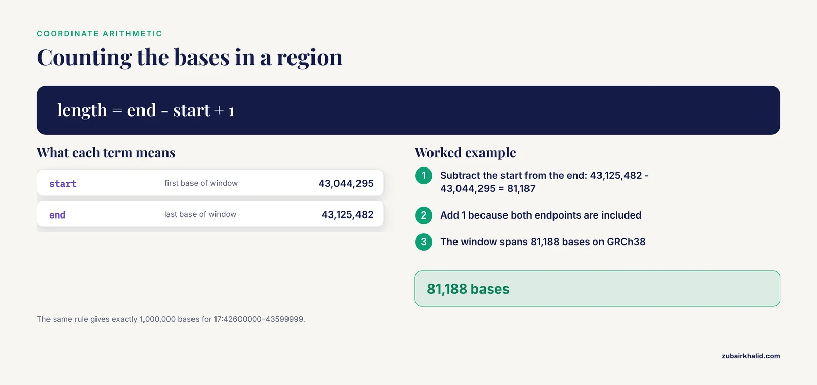
The coordinate system. The x-axis is position on the reference assembly. Ensembl coordinates are 1-based and inclusive, so a region written 17:43044295-43125482 includes both endpoints and spans 43,125,482 minus 43,044,295 plus 1, which is 81,188 bases. Positions count from the start of the assembled chromosome, not from a cytogenetic band, which is why the search box wants coordinates rather than band names whenever precision matters.
Layered companion databases. The gene track comes from the core schema. Variation tracks draw on imported public variant resources. Regulation tracks draw on large-scale functional genomics projects. Comparative tracks draw on Ensembl Compara, the database that stores homology calls, whole-genome alignments, and gene trees [4]. Each source is an independent layer you can switch on or off, and the view simply stacks whichever layers are active.
Rendering. The browser draws each track separately, historically as server-rendered image tiles and in the current interface largely as JavaScript graphics in your browser. Because tracks render independently, you can toggle any of them without touching the underlying annotation, and wide windows stay usable.
Third-party annotation through DAS. The Distributed Annotation System, DAS, is a protocol for serving annotation over the web so that a remote server's features can be drawn as extra tracks in someone else's browser. Statistical Viewer used DAS tracts to display uploaded feature annotation alongside its study-specific plots [3]. The pattern still describes how the view thinks about data: your data becomes one more track, aligned by coordinate.
Releases and archives. Ensembl updates its annotation on a regular release cycle, several times per year, and the main site always shows the current release. Archive sites freeze older releases so that published analyses remain reproducible, which matters because gene models and track contents change between releases [1]. Non-vertebrate species are served through the companion Ensembl Genomes resource, which follows the same browsing model.
How to Use Ensembl: Reaching Region in Detail, Step by Step
Work through these steps once at a real keyboard and the navigation becomes automatic.
- Open the browser and confirm the species and assembly. Go to the Ensembl website, select human, and read the assembly label on the page. Current human annotation sits on GRCh38. If you are reproducing an older analysis on GRCh37, start from the archive site for that assembly instead.
- Search for your region. The search box accepts gene symbols, variant identifiers such as rs numbers, and raw coordinates. Type BRCA1, or paste coordinates in the chromosome:start-end format with no thousands separators, for example 17:43044295-43125482. The search is assembly-aware, so the same query returns different windows on different assemblies.
- Read the three panels. You land on the Location tab. The ideogram at the top shows chromosome 17 with a red box around your window. Region in detail below it draws the annotated tracks. If the window is small enough, the sequence panel appears underneath.
- Frame the window you actually want. A gene search opens a window centered on the gene. For a controlled view, type coordinates. BRCA1 occupies about 81 kb on the minus strand of chromosome 17, at 17:43044295-43125482 in GRCh38. To read it with genomic context, enter 17:42600000-43599999, which is exactly 1,000,000 bases under inclusive counting and contains the gene with several hundred kilobases of flanking sequence on each side.
- Pan and zoom. Drag inside the detail view to slide along the chromosome, or drag across the tracks to select and zoom into a smaller span. The zoom controls widen and narrow the window. Click a cytoband in the ideogram to jump the view to that band. The address bar carries the coordinates in an r parameter, so a URL of the form ensembl.org/Homo_sapiens/Location/View?r=17:42600000-43599999 reproduces your exact window on any machine.
- Configure the tracks. Open Configure this page in the left-hand menu. Track categories cover genes, variation, regulation, comparative genomics, repeats, and more. Switch on what your question needs, for example the merged human gene set, variation, and conservation, and switch off the rest to cut clutter.
- Inspect a feature. Click any transcript. A report page opens with the exon structure, transcript and protein sequences, functional domains, and cross-references to other databases. Click a variant for alleles, population frequencies, and clinical annotation where public resources supply them.
- Export the window. The Export data link outputs the exact displayed region in standard formats, including FASTA for sequence and GFF for annotation, with additional tabular and formatted options. For anything beyond a quick copy, prefer the programmatic routes described below.
- Use the sibling tabs as complements. Tabs such as Genes, Variation, and Comparative genomics reframe the same coordinates as tables, lists, and summaries. Region in Detail remains the panel that ties them all to a single visual frame.
Reading the Tracks: Region in Detail Interpretation
Region in Detail interpretation is mostly pattern recognition: knowing what each drawing convention means and what question each track answers.
Gene and transcript tracks
Each transcript is drawn as blocks connected by lines. Filled blocks are exons. The wide filled portion marks the protein-coding part of each exon, and narrower blocks mark the untranslated regions at the ends. The connecting lines are introns, and small chevrons on those lines point in the direction of transcription. A gene on the minus strand is drawn with chevrons pointing left, and its transcripts read right to left across the window.
Expect more than one transcript per gene. Alternative splicing is the norm in vertebrate genomes, and the track stacks every annotated isoform for the same locus. For human and mouse, the merged Ensembl and GENCODE gene set is the standard reference annotation, and RefSeq models can be displayed alongside it for comparison. These gene sets are built by different pipelines from overlapping evidence, so their isoform lists and exon boundaries often differ. Ensembl's models come from automated, evidence-based annotation rather than per-gene manual curation [1], which makes them broad and regularly updated, and also means a given model can change between releases. When a paper refers to the canonical transcript, it means the isoform Ensembl flags as representative for the gene.
Two practical habits follow. First, always check which isoform your variant or primer actually hits, because an exon in one transcript can be an intron in another. Second, read the strand label before interpreting anything directional, including the basepair view.
Variation tracks
Switch on variation and the window fills with single nucleotide variants, short insertions and deletions, and, where annotated, larger structural variants. Colors group variants by predicted consequence class, such as coding change, intronic, or intergenic. Clicking a variant opens a page with its alleles, population frequencies, and clinical significance where public resources provide them. In gene-dense regions the track looks nearly solid. High density tells you the region is variable, not that anything is pathogenic. Pathogenicity is a judgment you make after opening the records, not a property of the color.
Regulation tracks
Regulatory tracks show promoters, enhancers, transcription factor binding sites, and insulator-type features such as CTCF binding, drawn from large-scale functional genomics projects. These features are computational integrations of experimental signals, and they are tissue-specific by construction. An enhancer drawn over your gene's first intron is a hypothesis supported by mapped signal in some cell type. It is not a proven functional element for your tissue until evidence supports that step.
Comparative genomics tracks
Conservation tracks score how strongly other species align to your window, base by base or block by block. Highly conserved noncoding stretches inside introns often flag functional elements worth checking. Alignment and synteny views show where orthologous sequence, that is, homologous sequence descended from a common ancestor, sits in other genomes. Ensembl Compara stores the underlying homology calls, alignments, and gene trees [4], and specialized browsers build directly on that data to compare gene structure across species, as described in the workflows section.
Repeats, RNA genes, and evidence tracks
Additional track categories round out the picture. Repeat annotation marks repetitive sequence that complicates read mapping and primer design. RNA gene tracks show structured RNAs separate from the protein-coding models. Evidence tracks display the cDNA, EST, and protein supports that the gene-building pipeline used, which helps you judge how well supported a given exon is [1].
The basepair view
Zoom until the window is a few kilobases wide and the sequence panel appears at the bottom. It shows the nucleotide sequence of the forward strand with a six-frame translation, meaning the sequence is translated in all three reading frames on each strand and displayed at once. Start and stop codons, splice signals, and overlapping variants are marked in context. This is the level where you confirm which codon a variant hits, check a splice site, or copy exact sequence for primer design. Remember the strand: the panel shows the forward strand of the assembly unless you reverse it.
A worked interpretation
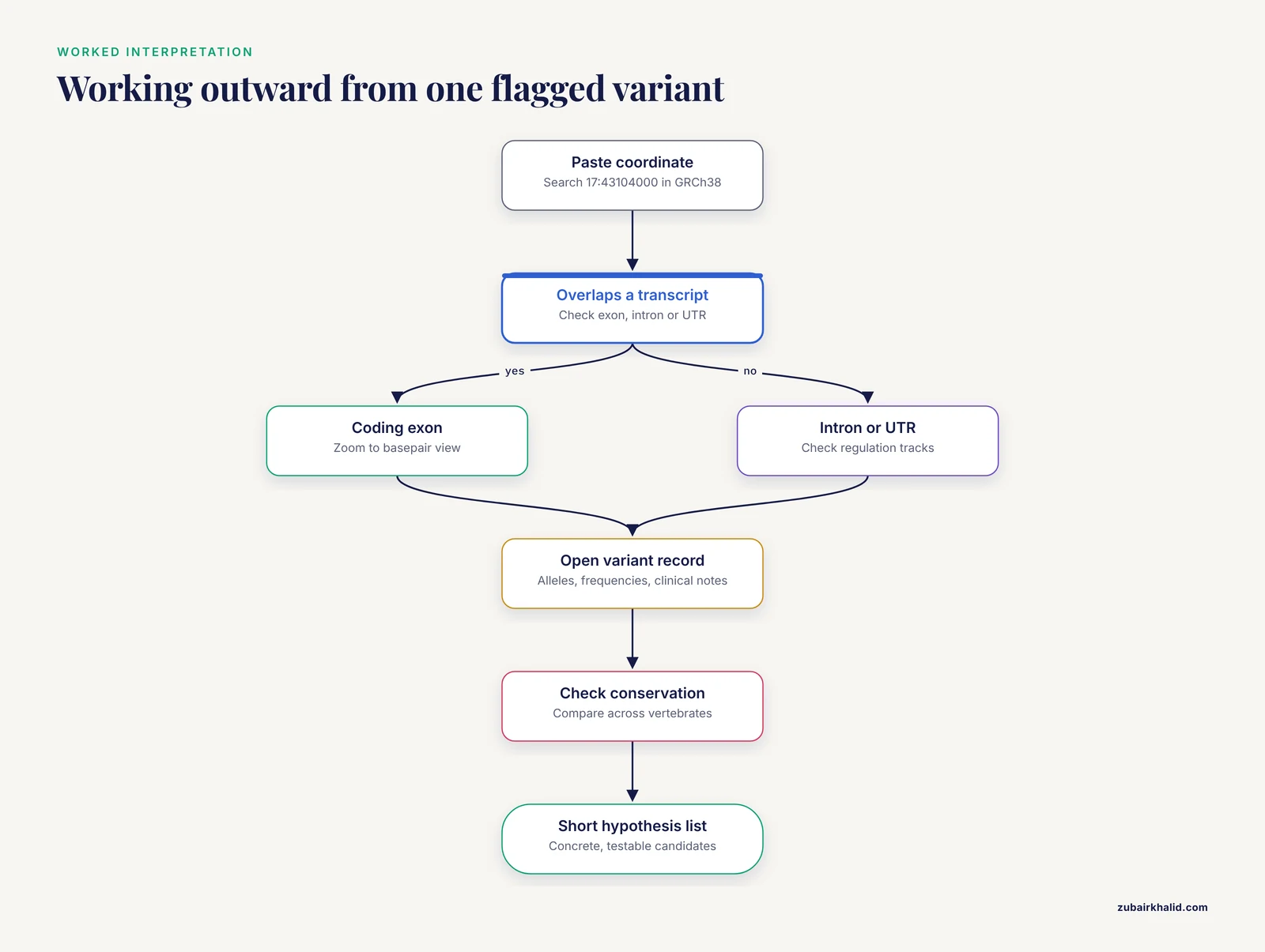
Suppose a variant-calling pipeline flags a single nucleotide variant at 17:43104000 in GRCh38, a hypothetical coordinate chosen because it falls inside the BRCA1 span, and you need to know what it touches. Paste the coordinate into the search box. The ideogram confirms the position at 17q21.31. In Region in detail, the variant marker falls within the BRCA1 gene body. Now work outward:
- Check which transcripts overlap the position, and whether it lands in an exon, an intron, or an untranslated region of each isoform.
- If any transcript places it in a coding exon, zoom to the basepair view and read the six-frame translation to see what the codon becomes.
- Open the variant record to check whether it is already cataloged, with population frequencies and any clinical annotation.
- Check conservation at that base across vertebrates.
- Check the regulation tracks, because an intronic variant may act through an overlapping regulatory element rather than through the transcript sequence.
Five clicks turn an anonymous coordinate into a short list of concrete, testable hypotheses. That is the core skill the view teaches, and it is the same skill that clinical and research workflows rely on.
Adding Your Own Data and Configuring the View
The built-in tracks answer background questions. Your own data answers your question, and the view accepts it in several ways.
File upload. The browser accepts standard formats such as BED (Browser Extensible Data) and GFF (General Feature Format) for annotation, and VCF (Variant Call Format) for variants, through its upload interface. A BED file of ChIP-seq peaks or a VCF of your called variants appears as a new track aligned by coordinate. Keep uploaded files modest in size for the web interface and move to track hubs for large data.
Track hubs. A track hub is a bundle of remote tracks described by a small set of configuration files, built for large datasets such as whole-genome alignments or genome-wide signal tracks. Register the hub URL once and its tracks appear in Region in Detail like built-in ones, remaining available across sessions. Laboratories use hubs to share figure-ready data with collaborators, because everyone sees the same tracks against the same assembly.
DAS sources. Legacy integrations publish annotation through DAS, which draws remote features as extra tracks. The Statistical Viewer upload server accepted statistical data and feature annotation in Excel form and displayed the annotation in DAS tracts [3]. DAS has been largely superseded by track hubs and APIs, but the design idea, remote annotation drawn in coordinate context, is the same one track hubs implement.
Sequence placement. If you hold a sequence of unknown position, run the built-in BLAST tool against the assembly. The report links each hit straight back into the browser at those coordinates.
Variant annotation. The Variant Effect Predictor, VEP, annotates your variants against the current Ensembl transcript set and returns standard consequence terms. Viewing VEP output in the region context shows immediately which isoforms share a consequence and which disagree.
Export and programmatic access. For bulk work, skip the picture. The REST API serves sequence and annotation for any region over HTTP, BioMart builds tabular queries across the databases, and the Perl API reads the core schema directly [1]. The view is for reading. Pipelines are for measuring.
Region in Detail in Real Research Workflows
The panel earns its keep inside larger workflows. Four examples show the range.
Clinical copy number interpretation. DECIPHER is an online repository of genotype and phenotype data used to interpret copy number variants, deletions and duplications that change gene dosage, in developmental disorders. Its published protocol has the clinician search for consented patients sharing a chromosomal location, navigate the region of interest with visualization tools and the Ensembl genome browser, analyze the affected genes, prioritize them by likelihood of haploinsufficiency, meaning the gene cannot function with only one working copy, and create printouts at different levels of detail [2]. That phrase, different levels of detail, is the overview to detail to basepair hierarchy put to clinical use. The browser panel is where a reported deletion becomes a ranked list of candidate genes.
From linkage peaks to candidate genes. Statistical Viewer extended Ensembl to prioritize candidate genes inside linkage regions for association analysis. The plug-in drew study-specific LOD score plots, LOD being the logarithm-of-odds statistic that measures linkage evidence at each marker, in a panel directly under the ideogram on Contig View and Cyto View pages, synchronized with a vertical sliding selection box, and its Get Map module converted markers' genetic map positions into genomic coordinates [3]. The design principle still stands: put your study's statistics on the same coordinate axis as the annotation, then read the overlap in a regional view.
Comparative gene structure. Aequatus is an open-source homology browser that provides an in-depth view of gene structure across gene families, built on precalculated alignment and feature data held in the Ensembl Compara and Core databases [4]. It goes below the gene level that standard synteny displays reach, down to conservation of individual exon boundaries among multiple genomes, and ships as a JavaScript module usable inside the Galaxy platform's GeneSeqToFamily workflow. Where Region in Detail shows one genome's window, this class of tool shows that window's evolutionary history.
Species-scale portals. Whole-genome portals wrap the same regional browsing idea around organism-specific data. GEGA, a chicken gene atlas, integrates the NCBI-RefSeq and EMBL-Ensembl/GENCODE catalogs on the GRCg7b assembly into 78,323 genes, including 24,102 protein-coding genes and 44,428 long non-coding RNAs, and layers expression profiles across 47 tissues from 36 datasets and 1,400 samples, with dedicated views for exploring a quantitative trait locus (QTL) region [5]. Xenbase, the Xenopus model organism database, hosts current and archived genomes for X. laevis and X. tropicalis with BLAST and GBrowse tools, and links its curated gene pages out to Ensembl [6]. In both cases the regional view is the bridge between a locus of interest and the annotation that explains it.
Annotation as ground truth. Large-scale gene discovery pipelines use Ensembl annotation to check their predictions. An iterative machine learning approach that discovered variable (V) exon genes, which encode the antigen-binding regions of B and T lymphocyte receptors, across whole genome shotgun datasets from 14 primate species validated its calls against Ensembl annotations [7]. The pattern generalizes to any method that claims to find features in a genome: the first sanity check is to place those features in their regional context against the standard annotation.
Common Mistakes and Limitations
These are the errors that cost people real time, listed so you can check for them before they happen.
Mixing assemblies. GRCh37 and GRCh38 coordinates differ for the same biological position, occasionally by large distances. A coordinate lifted from an older paper into the current browser can land in the wrong place entirely. Check the assembly label on every page, and use the archive site when reproducing analyses on GRCh37.
Measuring with your eyes. The view compresses long introns and wide gaps so features fit the window. Two exons that look adjacent can be tens of kilobases apart. Read every distance from coordinates or from exported data, never from the drawing.
Ignoring strand. Minus-strand genes are drawn right to left. Designing primers or reading the basepair view without checking the strand label can hand you the reverse complement of what you intended.
Treating one gene model as the truth. Ensembl, GENCODE, and RefSeq models differ in isoform lists and exon boundaries because they come from different automated pipelines, and Ensembl's annotation is explicitly a first-pass, evidence-based system [1]. Models change between releases. Record the release number and assembly with every figure.
Overreading prediction tracks. Regulatory features, consequence colors, and conservation scores are computational predictions layered on experimental signal. They generate hypotheses. They do not confirm function in your tissue or condition.
Analyzing the image. The view renders data but does not compute anything. Counts, lengths, overlaps, and statistics belong in exported data or API queries. Never count exons off a screenshot for anything that matters.
Zooming past the useful range. Whole-chromosome windows drop most detail. Use the Region overview for orientation, Region in Detail for reading, and the basepair view for sequence-level questions.
Forgetting configuration in shared figures. A screenshot without the assembly, release, coordinates, and active track list is not reproducible. Those four items belong in every figure legend, and the r parameter URL is the cleanest way to record the coordinates.
Quick Review
- Region in Detail is the middle panel of the Ensembl Location page, between the Region overview ideogram and the high-zoom basepair view.
- A region is a coordinate span on a reference assembly, written chromosome:start-end, with GRCh38 the current human assembly and coordinates 1-based and inclusive.
- Tracks are database renderings: genes, variation, regulation, comparative genomics, repeats, plus your own uploads, track hubs, and DAS sources [3].
- Introns are compressed. Distances come from coordinates, never from the drawing.
- Gene models differ between Ensembl, GENCODE, and RefSeq because they come from different automated pipelines [1].
- Click any feature for its report page, use Configure this page for tracks, and Export data for the exact window.
- Every figure needs the assembly, release, coordinates, and track list to be reproducible.
Frequently Asked Questions
What does the Ensembl Region in Detail view mean?
It is the main annotated, coordinate-based panel of the Ensembl genome browser, showing your chosen chromosome window as layered tracks of genes, variants, regulatory features, and comparative data. It is the middle level of the Location page, between the whole-chromosome overview and the basepair sequence view.
How do I open the Region in Detail view in Ensembl?
Search for a gene symbol, variant identifier, or coordinate range such as 17:43044295-43125482, then open the Location tab. The middle panel, labeled Region in detail, is the view. Configure this page controls which tracks it draws.
Why do introns look shorter than they really are?
The browser compresses long introns so a gene fits in the window. Exon and intron lengths must be read from coordinates or from the Export data output, never estimated from the drawing.
Can I add my own data to the Region in Detail view?
Yes. Upload BED, GFF, or VCF files through the browser interface, attach track hubs for large remote datasets, or add DAS sources for legacy annotation. Your data appears as extra tracks aligned by coordinate alongside the built-in annotation.
Is Region in Detail the same as the old ContigView?
Yes, it is the modern replacement. Ensembl releases before the interface redesign called the detailed view ContigView, and older papers describing panels and plug-ins use that name for the same coordinate-window concept.
How do I download the sequence or annotation for the region I am viewing?
Use the Export data link, which outputs the exact displayed window in formats including FASTA and GFF. For bulk or scripted access to the same data, use the Ensembl REST API or BioMart instead of the browser.
Sources
- The Ensembl automatic gene annotation system.
- Interpretation of genomic copy number variants using DECIPHER.
- Statistical Viewer: a tool to upload and integrate linkage and association data as plots displayed within the Ensembl genome browser.
- Aequatus: an open-source homology browser.
- GEGA (Gallus Enriched Gene Annotation): an online tool providing genomics and functional information across 47 tissues for a chicken gene-enriched atlas gathering Ensembl and Refseq genome annotations.
- Navigating Xenbase: An Integrated Xenopus Genomics and Gene Expression Database.
- Iterative Variable Gene Discovery from Whole Genome Sequencing with a Bootstrapped Multiresolution Algorithm.