How to Download RNA-Seq Raw Data from NCBI SRA: A Practical Guide
By Dr. Zubair Khalid, DVM, MS, PhD ·

By the end of this guide you will be able to locate an RNA-seq study on the NCBI website, identify the correct accession numbers, install the SRA Toolkit, download the raw sequencing runs, convert them to gzipped FASTQ files split by mate, and verify that the files are complete and usable for downstream analysis. Everything runs on a standard laptop or a modest cloud instance. The only software you need is the SRA Toolkit, which the authors of published RNA-seq pipelines use as the standard loading step before alignment and differential expression analysis [1][2].
Raw RNA-seq data are reads from the sequencer, before alignment, trimming, or counting. Public repositories store these reads so that any analysis can be reproduced or reanalyzed. A recent workflow protocol describes the full path, from downloading raw data through quality control, trimming, alignment, counting, and differential expression, and it starts with retrieving data from NCBI GEO and SRA [2]. This guide covers that first retrieval step in detail, because it is where most newcomers lose hours to small, avoidable problems.
You will need:
- A terminal (Terminal on macOS and Linux, PowerShell or Windows Terminal on Windows, or a cloud shell such as Google Colab, which one published protocol uses to run the entire RNA-seq workflow on free cloud resources [2])
- At least 10 GB of free disk space for a single run, and far more for a full study
- The SRA Toolkit installed (covered below)
- The accession number of the study or runs you want
How NCBI Organizes RNA-Seq Data
Before you download anything, you need to understand how to use NCBI and how its databases fit together. NCBI, the National Center for Biotechnology Information, maintains several linked databases. For RNA-seq, five matter:
- SRA (Sequence Read Archive) stores the raw sequencing reads. This is where the FASTQ-equivalent data live. One review of transcriptomic data acquisition notes that raw reads for RNA-seq experiments are generally available in the NCBI SRA, which is a large part of why reanalysis of RNA-seq studies is practical at scale [3].
- GEO (Gene Expression Omnibus) stores expression studies. For RNA-seq, GEO usually holds the processed data (gene count matrices, and sometimes normalized tables) and links to the raw reads in SRA. Many recent studies deposit both, for example raw reads plus counts and pathway statistics in GEO [4], or a GEO accession with processed expression profiles hosted separately [5].
- BioProject stores the study-level record, with an accession of the form PRJNA followed by digits, such as PRJNA1456794.
- BioSample stores sample-level metadata, with accessions like SAMN57450602. This is where you find tissue, treatment, and strain descriptions.
- TSA (Transcriptome Shotgun Assembly) stores assembled transcriptomes that some authors deposit alongside their reads [6].
The accession hierarchy matters because each level answers a different question. A BioProject describes the whole study. A BioSample describes one biological sample. An SRA run, with an accession like SRR38280322, is one sequencing lane or flow-cell section and is the unit you actually download. A GEO series, with a GSE accession like GSE292409, wraps the study with author-processed results. If you search NCBI for a paper's GSE accession and click through to the SRA links, you land on the same runs you would find through the BioProject. Real examples of this linkage appear throughout the literature: one single-cell kidney study cites the GEO accession GSE176155 together with the BioProject PRJNA735197 for the same underlying data [8], and a bacterial transcriptome dataset lists its SRA study accession SRP695241 alongside its BioProject PRJNA1456794 and run accessions SRR38280322 through SRR38280329 [9].
A key practical point from the data-integration literature: submitters deposit transcriptomic datasets with little standardization of format, so retrieving raw data can become complicated as the number of experiments grows [3]. Knowing the accession hierarchy keeps that complication manageable.
Step 1: Find the Dataset on the NCBI Website
If you have an accession from a paper, start there. If you are searching by topic, use the NCBI SRA or GEO search boxes directly.
From a paper accession
Most RNA-seq papers list an accession in the Data Availability section. A blueberry transcriptome study, for example, states that all raw reads were deposited in the NCBI SRA under run accessions SRR6281886, SRR6281887, SRR6281888, and SRR6281889 [6]. To find those runs:
- Go to the NCBI SRA search page and paste
SRR6281886into the search box. - The result page shows the run, its BioSample, its BioProject, the platform (Illumina in this case), and the read layout.
- Click the BioProject link to see every run in the study at once.
Searching by topic
- On the NCBI home page, open the SRA database from the dropdown or go to the SRA search directly.
- Search with descriptive terms, for example
"Zea mays" RNA-seq mycorrhiza, or a taxon plus a condition. - Use the "Species" and "Source" filters on the left. For RNA-seq you generally want "TRANSCRIPTOMIC" under Source.
- Open the "Send to" menu and choose "Run Selector" to view all runs in a study in a table with library layout, platform, and metadata columns.
- Tick the checkboxes for the runs you want and record their SRR accessions, either by hand or with the "Selected" export.
The Run Selector view is where you confirm the two details that decide your conversion command later: the library layout (paired vs. single) and whether the library is stranded. A maize dataset deposited with the QuantSeq 3' mRNA-Seq kit, for instance, is strand-specific 3'-end counting, and that fact changes how you interpret and analyze the reads later [10].
Grab the accession list
From the Run Selector, select your runs and use the export to save the SRR accessions. Alternatively, copy them into a plain text file on your computer. For the bacterial example dataset that file would contain eight lines [9]:
SRR38280322
SRR38280323
SRR38280324
SRR38280325
SRR38280326
SRR38280327
SRR38280328
SRR38280329
Save it as srr_list.txt. Every later step uses this list.
Step 2: Install and Configure the SRA Toolkit
The SRA Toolkit is NCBI's official command-line software for fetching and converting SRA data. Published pipelines rely on it as the loading stage of RNA-seq analysis [1], and protocol-level guides list it as the tool for extracting raw data from NCBI GEO and SRA [2]. The toolkit is maintained as open source, and multi-study transcriptomic projects have used its fasterq-dump tool to download data from 18 separate GEO studies for a single integrated analysis [11].
Install with whichever method matches your system:
# Recommended on any system with conda or mamba
mamba install -c bioconda sra-tools

# Ubuntu or Debian
sudo apt-get install sra-tools

# macOS with Homebrew
brew install sra-tools
The bioconda route is the safest because it installs a current version. Older toolkit versions bundled with some system repositories contain bugs that were fixed in later releases, and an outdated version is one of the most common causes of confusing download errors.
Verify the installation:
prefetch --version
fasterq-dump --version
Expected output looks like:
prefetch: 3.2.1
fasterq-dump: 3.2.1
If either command returns "command not found", your PATH does not include the installation directory. With conda, activate the environment first with conda activate your_env_name. Path and dependency problems like this are exactly the class of issues that RNA-seq troubleshooting guides flag as the most frequent setup stumbling blocks [2].
No configuration is required for public data in current toolkit versions. If you want to change where cached files are stored, run vdb-config, interactive and set the cache location. For most users the defaults are fine.
Step-by-Step: How to Download RNA-Seq Raw Data from NCBI SRA
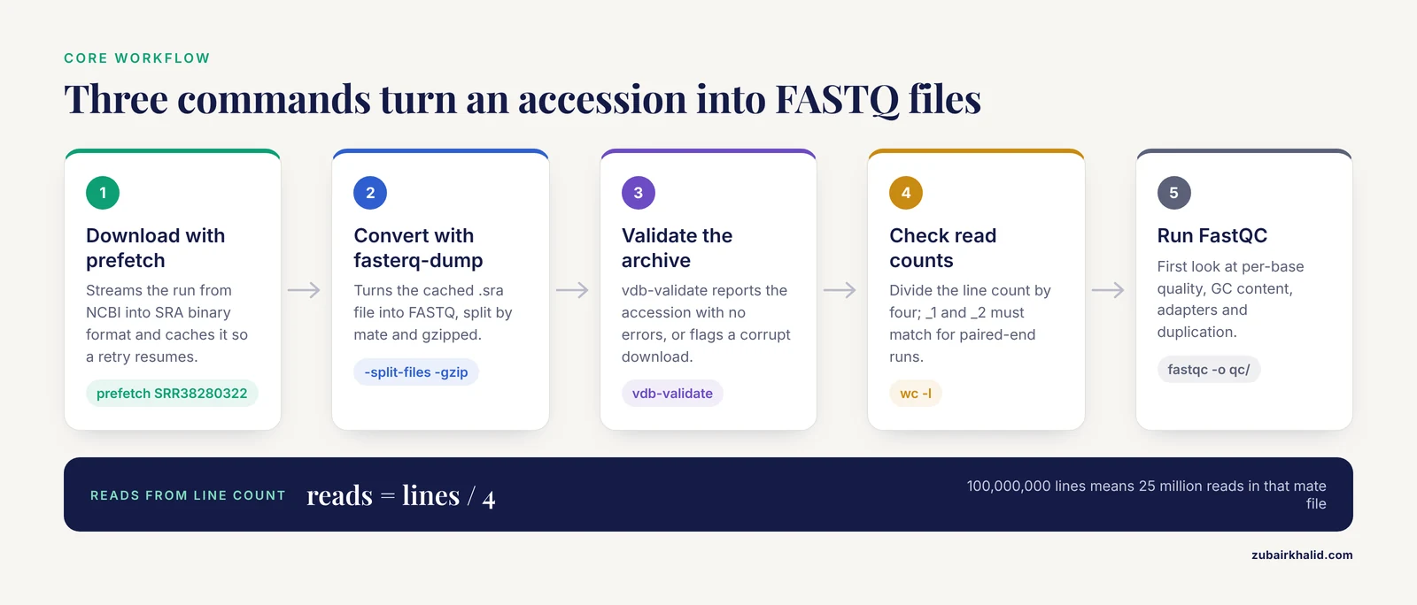
With the toolkit installed, the core workflow has three commands per run: prefetch downloads the run, fasterq-dump converts it to FASTQ, and vdb-validate confirms integrity. The following walkthrough uses one run from the freshwater bacterial dataset, SRR38280322, which is one of eight paired-end libraries totaling 349,853,404 processed reads [9].
Step 3: Download a run with prefetch
Set up a clean directory structure first:
mkdir -p rna-seq-project/sra rna-seq-project/fastq rna-seq-project/qc
cd rna-seq-project
Download the run:
prefetch SRR38280322 -O sraWhat happens: prefetch contacts NCBI, streams the run from the archive, and writes it in SRA's internal binary format. The -O sra option places the output under the sra folder instead of your current directory. On success the command returns quietly, and the file sits at sra/SRR38280322/SRR38280322.sra. Confirm with:
ls -lh sra/SRR38280322/Expected output, with a size that depends on the run's depth:
total 1.2G
-rw-r--r-- 1 user user 1.2G Nov 11 10:04 SRR38280322.sra
Why prefetch instead of converting directly? Two reasons. First, prefetch stores the run in a local cache, so if conversion is interrupted you can retry fasterq-dump without re-downloading. Second, prefetch handles interrupted network transfers gracefully, so rerunning the same command picks up where it left off rather than starting over.
One parameter to know: prefetch applies a default maximum size cap for a single run. If a run is larger than the cap, the tool stops and prints a message telling you the size limit was reached. Raise the cap with -max-size, for example prefetch SRR38280322 -O sra, max-size 50G. Most RNA-seq runs are far below this cap, but deep long-read or large-scale runs can hit it.
Step 4: Convert SRA to FASTQ with fasterq-dump
SRA files are not FASTQ. SRA is a compressed binary format that stores reads, quality scores, and metadata. Every analysis tool you will use, from FastQC to the aligner, expects FASTQ, which stores each read as four lines: a read name starting with @, the sequence, a separator line starting with +, and per-base quality scores encoded in Phred+33 characters. Conversion is therefore mandatory.
fasterq-dump sra/SRR38280322/SRR38280322.sra \
  -O fastq \
  --split-files \
  --gzip \
  --threads 6
(The backslashes just continue the command onto multiple lines for readability. Type it as one line if you prefer.)
For a paired-end run this produces two files:
fastq/SRR38280322_1.fastq.gz
fastq/SRR38280322_2.fastq.gz
_1 holds read 1 of each pair and _2 holds read 2. For a single-end run you get one file, fastq/SRR38280322.fastq.gz.
Each flag matters:
-split-fileswrites forward and reverse mates to separate files. Without it, fasterq-dump writes one file per spot, which most aligners cannot consume directly.-gzipcompresses the output. Uncompressed FASTQ for a mammalian run can run tens of gigabytes, and gzip typically cuts that to roughly a third of the size with no loss.-O fastqsets the output directory.-threads 6uses six threads. fasterq-dump is multithreaded and much faster than the olderfastq-dumptool, which is one reason recent pipelines use it for bulk retrieval [11]. Match the thread count roughly to your available cores.
Peek at the output to confirm it is a sane FASTQ:
zcat fastq/SRR38280322_1.fastq.gz | head -n 8Expected output:
@SRR38280322.1 1 length=150
GATCGATCGG...
+SRR38280322.1 1 length=150
IIIIIIIIII...
@SRR38280322.2 1 length=150
...
Every read must occupy exactly four lines. If you see that pattern, the conversion worked.
Step 5: Download many runs in batch
Real studies have dozens of runs. The tomato salicylic acid dataset described in one Data in Brief article contains 12 SRA datasets from three biological replicates [12], and a sorghum stress dataset contains 54 strand-specific libraries [13]. Nobody does that by hand one run at a time.
With your srr_list.txt file in place:
# Download all runs, four at a time
xargs -a srr_list.txt -n 1 -P 4 prefetch -O sra

# Convert them all, one conversion at a time
while read acc
do
  fasterq-dump sra/$acc/$acc.sra -O fastq --split-files --gzip --threads 6
done < srr_list.txt
Notes on this batch block:
xargs -n 1 -P 4runs four prefetch jobs in parallel. More than four to six parallel downloads usually stops helping because you become limited by bandwidth, not by your CPU.- The
while readloop converts each run after download. Conversion is disk- and CPU-intensive, so running conversions one at a time is usually faster overall than running several in parallel against a single disk. - Add
echoinside the loop, as inecho Converting $acc, if you want a visible progress line per run.
Keep the srr_list.txt file in your project directory. It is your permanent record of exactly which runs belong to your analysis, and it makes the whole download reproducible with two commands.
Step 6: Verify the files are correct
Verification has three levels. Do all three before you invest hours in alignment.
First, validate the downloaded archive with the toolkit's own checker:
vdb-validate sra/SRR38280322/SRR38280322.sraA clean result reports the accession with no errors. Any "value error" or "read error" line means the download is incomplete or corrupt, and the fix is to delete the cached file and rerun prefetch.
Second, check read counts. FASTQ files have four lines per read, so divide the line count by four:
zcat fastq/SRR38280322_1.fastq.gz | wc -lIf the output is 100,000,000 lines, the run holds 25 million reads in that mate file. For a paired-end run, _1 and _2 must have identical line counts. If they differ, the conversion failed partway and you should rerun it.
Third, run a quality check on the FASTQ files. FastQC is the standard first look, and it is part of the published minimal-hardware RNA-seq workflow [2]:
fastqc fastq/*.fastq.gz -o qc/FastQC produces an HTML report per file showing per-base quality, GC content, adapter contamination, and sequence duplication. Per-base quality declining toward the ends of reads and visible adapter sequence are normal observations at this stage, and tools such as Trimmomatic, which the same workflow uses after download, address them [2].
Key Command Options at a Glance
| Tool | Option | What it does |
|---|---|---|
| prefetch | -O directory | Sets the download destination directory |
| prefetch | -max-size 50G | Raises the per-run size cap for large runs |
| prefetch | (cache) | Stores the .sra file so retries do not re-download |
| fasterq-dump | -split-files | Writes paired-end reads as two files, _1 and _2 |
| fasterq-dump | -gzip | Compresses FASTQ output, typically to about a third of the raw size |
| fasterq-dump | -O directory | Sets the FASTQ output directory |
| fasterq-dump | -threads N | Uses N threads for conversion |
| fasterq-dump | -temp directory | Redirects temporary files to a directory with more space |
| vdb-validate | accession | Confirms the downloaded archive is complete and undamaged |
Troubleshooting: Exact Errors and Fixes
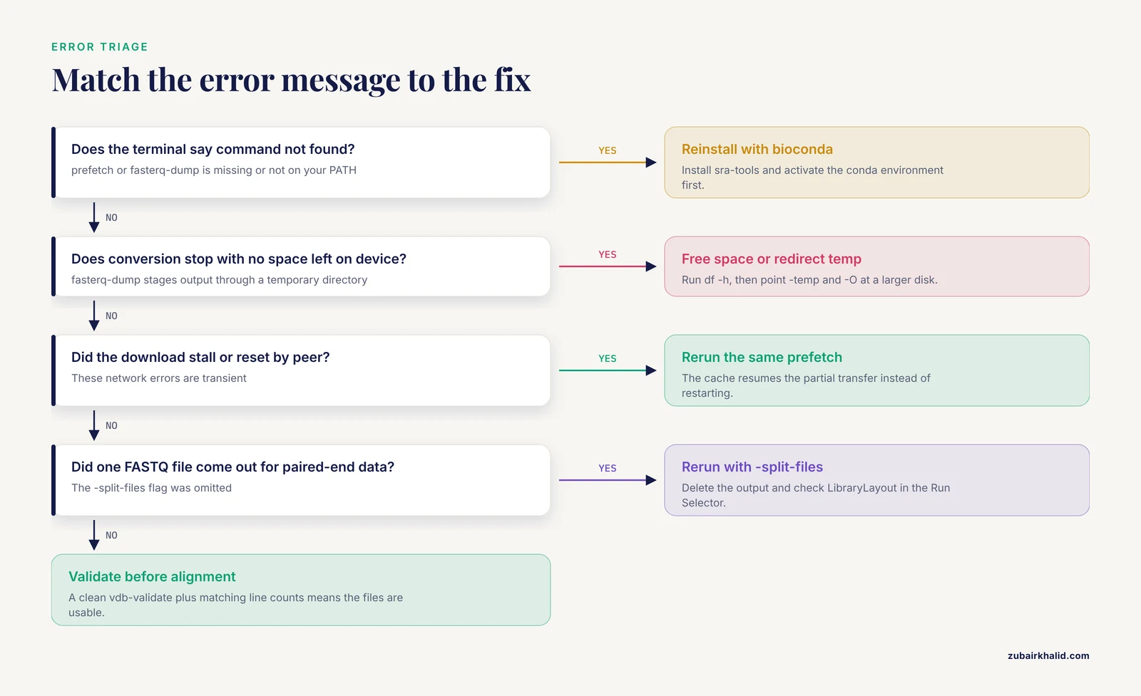
These are the errors you will actually hit, with their real messages and the fixes.
"command not found" for prefetch or fasterq-dump. The toolkit is not installed or not on your PATH. Reinstall with bioconda and activate the environment. Setup and path problems are the most commonly reported troubleshooting category in RNA-seq workflow protocols [2].
"No space left on device" during conversion. fasterq-dump stages its output through a temporary directory before writing the final files, and it needs roughly as much temp space as the uncompressed FASTQ will occupy. Run df -h to check free space. Either free space, or point conversion at a larger disk with -temp /path/to/big/disk, and use -O to send the final files there as well. On cloud platforms such as Google Colab, the published workflow attaches the working drive and runs the download there for exactly this reason [2].
Download stalls or ends with network errors such as "connection reset by peer". These are transient. Rerun the same prefetch command. Because prefetch caches partial transfers, the rerun resumes rather than restarting. If a specific run fails repeatedly, download it alone rather than in a batch so you can see the error clearly.
fasterq-dump reports the run cannot be found even though prefetch worked. You probably passed a path with a typo, or the cached file sits one directory deeper than expected. Run find sra -name "*.sra" to list the actual paths and pass them explicitly.
One FASTQ file came out for a paired-end run. You omitted -split-files. Delete the output and rerun with the flag. Check the layout in the SRA Run Selector before converting so you know what to expect. Some SRA records are genuinely single-end, and the Run Selector's LibraryLayout column tells you which is which.
Old toolkit versions fail with conversion errors that do not reproduce in coworkers' hands. Upgrade. Version skew is a known trap, and the fix is the bioconda install above. The SRA Toolkit is actively maintained open-source software hosted on GitHub.
Alignment later reveals very low mapping rates. The download was fine, but the reference genome is a poor match for your organism. A real example: in the four-isolate bacterial transcriptome dataset, alignment rates ranged from about 89 to 92 percent for three isolates but only 34.75 percent and 21.39 percent for the Micrococcus isolate, which the authors attribute to reference mismatch [9]. Nothing about that is a download failure, and it is the kind of issue you catch only by looking at the QC and mapping statistics after the data arrive.
Alternatives to the SRA Toolkit
Three other routes are worth knowing, each suited to a different situation.
Browser download of supplementary files. GEO often hosts processed data as supplementary files: gene count matrices, normalized tables, and sometimes the FASTQ files themselves. The zebrafish contaminant dataset deposited raw reads in GEO under GSE319292 alongside counts and enrichment statistics [4], and the hepatocyte population-variability dataset under GSE293032 provides the RNA-seq dataset with processed context [5]. If your question can be answered from a count matrix, downloading the processed supplementary files can save you days of compute. You lose the ability to redo QC, trimming, or alignment on your own terms, so make that trade deliberately.
Purpose-built acquisition tools. For projects that pull in many expression datasets, specialized acquisition tools exist. COMMAND>_ was designed specifically to simplify gene expression data acquisition across the heterogeneous formats that public repositories contain [3]. If your project involves many studies and multiple users, a dedicated tool reduces the bookkeeping that raw prefetch loops impose.
End-to-end pipelines that bundle the download. PipeSeq is an automated pipeline that packages the loading step with SRA Toolkit together with HISAT2 alignment, StringTie assembly, FeatureCounts counting, and DESeq2 statistics behind a simple visual interface [1]. If you want the download and everything after it in one place, this class of tool handles the retrieval for you. The trade is less control over the download commands themselves.
A useful habit from the deposition literature: check whether the authors also shared processed outputs elsewhere. The sorghum stress dataset, for example, deposited raw reads in SRA and hosted differential expression profiles, enrichment analyses, and a co-expression network on Figshare [13]. Retrieving both gives you raw and processed views of the same experiment.
What to Do After the Download
Downloading is step one of a longer chain. The standard sequence, as implemented in published workflows, is: quality control with FastQC, adapter and quality trimming with Trimmomatic, alignment to a reference genome with HISAT2 or BWA, format handling with Samtools, read counting with Subread's featureCounts, normalization, and differential expression with DESeq2 or pyDESeq2, followed by enrichment analysis with tools such as g:Profiler [2]. PipeSeq automates the same chain, from SRA Toolkit loading through HISAT2, StringTie, FeatureCounts, and DESeq2 [1].
Two downstream decisions connect directly back to what you downloaded.
Check the library type again. Stranded, 3'-end counting libraries such as those made with the QuantSeq kit [10] are counted differently from standard stranded total RNA libraries. Misreading the library type is a silent error that corrupts count-based statistics without producing any warning.
Plan for annotation before you plan for alignment. For non-model organisms, functional interpretation, not the download or the alignment, is usually the bottleneck. Recent work addresses this by building custom annotation R packages from NCBI genomic data so that enrichment analysis with clusterProfiler works even when curated annotations are scarce, demonstrated on Mycobacterium tuberculosis H37Rv [7]. If your organism is not well annotated, retrieval from NCBI does not stop at the FASTQ files.
Common Mistakes and Limitations
These are the mistakes that cost the most time, in the order they tend to happen.
Confusing accession levels. Downloading one SRR run and treating it as the whole study is the classic error. A study with 54 libraries [13] or 12 SRA datasets [12] cannot be reconstructed from a single run. Confirm the number of runs in the Run Selector before you start, and confirm your list length matches it.
Assuming the SRA record tells you everything about the samples. Metadata quality varies widely because submitters deposit with little enforced standardization [3]. Read the paper's methods, not just the SRA record, and cross-check BioSample entries. Strandedness, in particular, is frequently recorded incorrectly in SRA metadata, and the definitive answer often lives in the paper's methods section.
Underestimating disk space. A paired-end run at mammalian depth decompresses to multiple gigabytes of FASTQ, and fasterq-dump needs comparable temporary space on top of that. Batch downloads multiply the problem. Check df -h before a batch, not after the first "No space left on device".
Using single-end commands on paired-end data or vice versa. Without -split-files, paired-end data comes out in a form your aligner will reject or misinterpret. Check the LibraryLayout column in the Run Selector and use the right conversion flags every time.
Ignoring verification. A truncated FASTQ can pass visual inspection and fail silently days later during counting. vdb-validate, line-count checks, and FastQC are cheap. Rerunning an entire study after discovering a corrupt run mid-analysis is not.
Redownloading from scratch after every hiccup. The prefetch cache exists precisely so you do not have to. Delete and re-prefetch only when vdb-validate reports actual corruption.
Downloading raw data when processed data would answer the question. If the authors deposited count matrices in GEO [4][5] or hosted processed expression profiles on Figshare [13], and your analysis starts from counts, use them. Raw data matter when you need your own QC, trimming, alignment, or counting choices, or when the deposited processed data are incomplete.
One honest limitation applies to all public transcriptomic retrieval: you are trusting that the deposited raw reads match what the paper describes, and the only way to test that is to reproduce the authors' direction of effect from your own counts. Secondary analyses routinely and successfully reanalyze public RNA-seq data, from single-study reprojection to meta-analyses that batch-correct data downloaded from 18 GEO studies [11], so the trust is generally warranted, but it is earned through your own QC, not assumed.
Frequently Asked Questions
What is the difference between GEO and SRA?
GEO is the study-level expression database that holds processed results such as count matrices and links out to raw data, while SRA is the archive that stores the raw sequencing reads themselves. For an RNA-seq study you usually find the GSE accession in GEO, follow its links to the SRA runs, and download those runs for raw analysis [4][5].
Can I download SRA data without installing anything?
Yes, the SRA website offers browser downloads of the .sra file per run, but you still need the toolkit to convert that file to FASTQ, and you lose batching, caching, and resume capability. For anything beyond one or two runs, install the SRA Toolkit [2].
What is the difference between prefetch and fasterq-dump?
prefetch downloads the run from NCBI in SRA's binary format and caches it locally so interrupted downloads can resume, while fasterq-dump converts a cached .sra file into FASTQ. Running them in that order is the robust pattern, though fasterq-dump alone can stream directly from NCBI for a single run.
How do I download paired-end data as two FASTQ files?
Add -split-files to fasterq-dump, which writes the forward reads to a _1.fastq.gz file and the reverse reads to a _2.fastq.gz file. Confirm the library layout is paired in the SRA Run Selector first, and check afterward that both files have identical line counts.
How much disk space do I need for an RNA-seq download?
Plan for roughly a few gigabytes of compressed FASTQ per run plus a comparable amount of temporary space during conversion, and scale by the number of runs in your study list. Batch downloads of 8 to 54 runs, which are common sizes in published datasets, need tens to hundreds of gigabytes.
Why is my download so slow, and what can I do about it?
Most slowdowns come from bandwidth limits on a single connection, so run a few prefetch jobs in parallel with xargs -P rather than one huge stream. Rerun stalled prefetch commands rather than restarting from scratch, because the cache lets them resume.
How do I download an entire study's runs at once?
Collect the SRR accessions from the SRA Run Selector into a text file, then loop prefetch over that file with xargs -n 1 -P 4, followed by a conversion loop over the cached files. The two-command batch shown above reproduces the full download from the accession list alone.
What should I do right after the FASTQ files arrive?
Validate with vdb-validate, check read counts, and run FastQC before anything else. Then proceed to trimming, alignment with HISAT2, counting with featureCounts, and differential expression with DESeq2, following a published workflow order [2][1].
Sources
- Development and validation of the PipeSeq program for RNA-seq data analysis in the Chlamydomonas reinhardtii as a model.
- Streamline Protocol for Bulk-RNA Sequencing: From Data Extraction to Expression Analysis.
- First step toward gene expression data integration: transcriptomic data acquisition with COMMAND>_.
- Transcriptomic data of larval zebrafish exposed to environmentally relevant levels of uranyl nitrate and sodium arsenite.
- A comparative transcriptomic dataset of hepatocytes derived from a panel of human induced pluripotent stem cells with different ethnicities as an in vitro population variability toxicity model.
- Dataset of de novo assembly and functional annotation of the transcriptome of blueberry (Vaccinium spp.).
- Enhanced RNA-Seq Expression Profiling and Functional Enrichment in Non-model Organisms Using Custom Annotations.
- Expression analysis of epithelial membrane protein 1 (EMP1) gene in kidney stone patients.
- Transcriptome datasets of four freshwater bacterial isolates grown under iron-replete and iron-limited conditions.
- Illumina RNA-seq data of Genotype-specific responses of maize plants to Funneliformis mosseae.
- A multi-omic analysis reveals the esophageal dysbiosis as the predominant trait of eosinophilic esophagitis.
- Transcriptome datasets of salicylic acid-treated tomato plant cultures under normal and stress conditions.
- A comprehensive transcriptomic dataset of Sorghum bicolor seedlings under abiotic stress conditions.