How to Download the Complete Human Genome from NCBI FTP
By Dr. Zubair Khalid, DVM, MS, PhD ·

By the end of this guide you will be able to download the complete human reference genome from NCBI, verify that the file arrived intact, confirm that the sequence content is what the accession promises, and prepare the FASTA for alignment or any other downstream analysis. Every command shown runs on a standard Linux or macOS shell. Windows users can run the same commands under WSL2.
Before you start, make sure you have:
- A Linux or macOS shell with
wget(orcurl) andmd5suminstalled.md5sumships with GNU coreutils. On macOS,md5 -qreplaces it, or install coreutils with Homebrew. - About 10 GB of free disk space. The compressed genome FASTA is close to 1 GB, the decompressed FASTA is a little over 3 GB, and an alignment index roughly triples that again.
- Optionally, the NCBI
datasetscommand-line tool, which offers a friendlier programmatic route to the same data [1]. - A stable network connection. A resumed download beats a restarted one, so this guide uses
wget -candrsyncthroughout.
Why NCBI FTP and Which Files You Actually Need
NCBI maintains two parallel versions of every genome assembly. RefSeq records are curated by NCBI staff and carry GCF_ accession prefixes, while GenBank records are submitter-provided and carry GCA_ prefixes. RefSeq has served as the curated human genome resource at NCBI since its introduction in 2000, and for the human reference the RefSeq version (GCF) is what most alignment tools, annotation tracks, and clinical pipelines expect [2].
The human reference itself is produced by the Genome Reference Consortium (GRC), whose stated mission is to improve the human reference assembly by correcting errors and adding sequence so it best represents the human genome for basic and clinical research. GRC data flows into the three major genome browsers, UCSC, Ensembl, and NCBI, and those browsers are the source of most of the confusion between differently named but equivalent files [3]. When you download human genome data from NCBI FTP, you are getting the GRC assembly packaged in RefSeq form.
For a complete, analysis-ready download you want one assembly directory that contains:
- The genome sequence itself as FASTA (
*_genomic.fna.gz), which includes the chromosomes, unplaced and unlocalized scaffolds, and alternate loci. - The annotation (GFF3 or GenBank flat file), if you plan to interpret features rather than just align reads.
- The
assembly_report.txtandassembly_stats.txt, which tell you exactly what is in the FASTA. - The
md5checksums.txt, which lets you prove the download is bit-for-bit correct.
There is also a newer access route worth knowing. NCBI Datasets wraps taxonomy, gene, and genome data behind a unified interface with command-line tools and APIs, and recent updates extended programmatic taxonomy access and improved the way taxonomic queries connect users to gene and genome data [1]. The datasets CLI is the quickest way to fetch a reference genome without hand-navigating directory trees, while raw FTP remains the right choice when you need every file in an assembly directory or want resumable mirroring.
How to Use NCBI: Finding the Current Reference Assembly
Assembly versions matter more than most people realize. GRCh37 and GRCh38 have different coordinates for the same variants, so a mismatch between your reference and your annotation or variant coordinates silently corrupts results. Before you download human genome data from NCBI FTP, confirm which assembly you want and which release is current.
The fastest check uses the datasets CLI. If you do not have it, install it through conda:
conda install -c conda-forge ncbi-datasets-cliThen ask for a summary of the current RefSeq reference genome for human:
datasets summary genome taxon "Homo sapiens" --referenceExpected output looks similar to this (trimmed for length):
{
    "reports": [{
        "accession": "GCF_000001405.40",
        "organism": {"taxon_id": 9606, "common_name": "human"},
        "assembly_info": {
            "assembly_level": "Chromosome",
            "assembly_name": "GRCh38.p14",
            "release_date": "2023-02-14"
        },
        "assembly_stats": {
            "total_sequence_length": "3344223425",
            "number_of_chromosomes": "25"
        }
    }]
}
The two fields that matter are the accession (GCF_000001405.40, the RefSeq representation of GRCh38 patch 14) and the total sequence length, which is about 3.34 gigabases once unplaced scaffolds and alternate loci are included. If a newer patch has been released by the time you read this, the accession suffix will differ, and the same command will show it. This is one of the core tips for anyone learning how to use NCBI: never hardcode an accession you have not confirmed against the live record.
Download Human Genome from NCBI FTP Step by Step
The following walkthrough covers three download methods in order of preference for most users, then verification and preparation. Any one of steps 2, 3, or 4 gets you the data. Steps 5 through 7 apply regardless of method.
Step 1: Create a Working Directory and Check Space
mkdir -p ~/genomes/human_grch38 && cd ~/genomes/human_grch38
df -h .
Expected output:
Filesystem      Size  Used Avail Use% Mounted on
/dev/nvme0n1p2  916G  214G  679G  24% .
If Avail shows less than about 15 GB, clear space or point the directory at a larger volume before continuing.
Step 2: Download with the NCBI Datasets CLI (Simplest Method)
This one command fetches the reference genome FASTA, gene annotation, and protein translations, already verified and packaged:
datasets download genome taxon "Homo sapiens" --reference \
  --include genome,gff3,gbff,protein \
  --filename human_grch38_refseq.zip
Parameters that matter:
-referencerestricts the result to the RefSeq reference assembly rather than every human assembly in the database.-includeselects file types.genomeis the FASTA,gff3is the annotation,gbffis the GenBank flat file with feature tables, andproteinadds translated proteins.-filenamenames the output archive.
Unpack it:
unzip human_grch38_refseq.zip
find ncbi_dataset -type f | head
Expected output:
ncbi_dataset/data/GCF_000001405.40/GCF_000001405.40_GRCh38.p14_genomic.fna
ncbi_dataset/data/GCF_000001405.40/genomic.gff
ncbi_dataset/data/GCF_000001405.40/sequence_report.jsonl
ncbi_dataset/data/dataset_catalog.json
The tradeoff is control. The CLI gives you a curated subset of files, not the complete assembly directory, and it does not hand you the NCBI md5checksums.txt. For many analyses the subset is exactly enough. For a fully reproducible pipeline that archives everything, use the FTP route below.
Step 3: Direct Download from NCBI FTP with wget
The canonical location for the human reference is the RefSeq vertebrate_mammalian tree. Set the base URL as a variable so the commands stay readable, then pull the files you need:
BASE="https://ftp.ncbi.nlm.nih.gov/genomes/refseq/vertebrate_mammalian/Homo_sapiens/all_refseq/GCF_000001405.40_GRCh38.p14"

wget -c "${BASE}/GCF_000001405.40_GRCh38.p14_genomic.fna.gz"
wget -c "${BASE}/GCF_000001405.40_GRCh38.p14_genomic.gff.gz"
wget -c "${BASE}/GCF_000001405.40_GRCh38.p14_assembly_report.txt"
wget -c "${BASE}/GCF_000001405.40_GRCh38.p14_assembly_stats.txt"
wget -c "${BASE}/md5checksums.txt"
Parameters that matter:
- The HTTPS prefix works on networks that block the FTP protocol, which is common on institutional firewalls.
https://ftp.ncbi.nlm.nih.gov/...,ftps://ftp.ncbi.nlm.nih.gov/..., andftp://ftp.ncbi.nlm.nih.gov/...all serve identical content. -c(continue) resumes an interrupted transfer instead of restarting from byte zero. On a file this size across a flaky connection, this flag is the difference between a 20-minute and a 3-hour download.md5checksums.txtsits at the top of theall_refseqdirectory and covers every release, which is why it is fetched separately from the release-specific files.
If you also want the full GenBank-format flat file with all features, add:
wget -c "${BASE}/GCF_000001405.40_GRCh38.p14_wgsmaster.gbff.gz"A direct listing of the directory is always available in a browser at the same HTTPS URL, which is a useful habit when you are unsure what a release contains.
Step 4: Mirror the Whole Assembly Directory with rsync
When you want every file in the release, including the GenBank flat file directory, CDS and protein translations, and the wgsmasta record, rsync mirrors the directory once and then only transfers differences on later runs:
rsync -avP \
  rsync://ftp.ncbi.nlm.nih.gov/genomes/refseq/vertebrate_mammalian/Homo_sapiens/all_refseq/GCF_000001405.40_GRCh38.p14/ \
  ./GCF_000001405.40_GRCh38.p14/
Parameters that matter:
-apreserves timestamps and permissions,-vreports progress per file, and-Penables partial transfers and resumption. Re-running the same command after an interruption picks up where it stopped.- The trailing slash on the source path means "copy the contents of this directory" rather than the directory itself. Getting this wrong is harmless here but produces nesting surprises elsewhere.
- Re-running rsync on a schedule is how you keep a local mirror current with minimal bandwidth.
Never rsync the parent vertebrate_mammalian/Homo_sapiens/ tree unless you genuinely want several hundred assemblies. The human directory contains every human assembly ever deposited, which is tens of terabytes.
Step 5: Verify the Download with MD5 Checksums
NCBI publishes an MD5 checksum for every file. Verification is not optional decoration. Interrupted transfers and mirrored caches occasionally produce corrupted files that fail only when a aligner hits a truncated record.
Because md5checksums.txt lists every file in the whole human release, filter it to the files you actually downloaded:
grep -E "GRCh38.p14_genomic.fna.gz|GRCh38.p14_genomic.gff.gz|GRCh38.p14_assembly_report" md5checksums.txt > local.md5
md5sum -c local.md5
Expected output:
GCF_000001405.40_GRCh38.p14_genomic.fna.gz: OK
GCF_000001405.40_GRCh38.p14_genomic.gff.gz: OK
GCF_000001405.40_GRCh38.p14_assembly_report.txt: OK
An OK on every line means the files match NCBI byte for byte. A FAILED line means the file is corrupted or incomplete. Delete the named file and re-run the download with -c; if the failure repeats, try the rsync route, which detects and repairs partial transfers natively.
Step 6: Decompress and Sanity-Check the Sequences
gunzip GCF_000001405.40_GRCh38.p14_genomic.fna.gzThen confirm the record count and total length:
grep -c '^>' GCF_000001405.40_GRCh38.p14_genomic.fnaExpected output (a value in this range, exact count varies with patches):
640samtools faidx GCF_000001405.40_GRCh38.p14_genomic.fna
awk '{s+=$2} END {print s}' GCF_000001405.40_GRCh38.p14_genomic.fna.faiExpected output:
3344223425That total matches the total_sequence_length reported by the datasets summary command in the earlier step, which is the cleanest cross-check available: two independent access routes agreeing on the same number. If you do not have samtools, the assembly_stats.txt file you downloaded reports the same totals, and NCBI Datasets exposes the same figures programmatically [1].
Inspect the first FASTA header so you know what identifiers look like:
head -n 1 GCF_000001405.40_GRCh38.p14_genomic.fnaExpected output:
>NC_000001.11 Homo sapiens chromosome 1, GRCh38.p14 Primary AssemblyTwo things stand out. First, RefSeq sequence identifiers are accessions like NC_000001.11, not chromosome names, and tools such as samtools faidx key on the first whitespace-delimited token. Second, this FASTA includes more than the 25 canonical chromosomes. The complete set contains unlocalized scaffolds (sequences known to belong to a chromosome but not ordered within it), unplaced scaffolds (not assigned to any chromosome), alternate loci (alternative representations of regions with excessive diversity, such as the MHC), and fixes from patches. The assembly_report.txt classifies every sequence with an assigned role, which is the authoritative key to this structure.
Step 7: Build an Alignment Index (Optional but Typical)
Most people downloading the genome intend to align reads. Two common indexers:
bwa index GCF_000001405.40_GRCh38.p14_genomic.fnaor for long reads:
minimap2 -d grch38.mmi GCF_000001405.40_GRCh38.p14_genomic.fnaIndexing takes tens of minutes on a typical workstation and consumes additional disk space, so plan for it in step 1. If your downstream plan is database searching rather than read alignment, indexing the human genome for BLAST-style k-mer lookup raises the same size considerations, and sampling strategies for k-mer indexes have been studied directly on the human genome to reduce index size and query time [4].
Key Files in the NCBI Assembly Directory
| File | What it contains | Typical use |
|---|---|---|
| , - | , - | , - |
*_genomic.fna.gz | All sequences, chromosomes plus unplaced, unlocalized, and alt scaffolds | Read alignment, sequence extraction |
*_genomic.gff.gz | Gene, transcript, exon, and CDS features in GFF3 format | Annotation overlap, QC of alignments |
*_wgsmaster.gbff.gz | Full GenBank flat file for the whole genome set | Feature tables, provenance, annotations |
*_protein.faa.gz | Translated protein products of annotated CDS | Protein search, functional annotation |
*_assembly_report.txt | Sequence-to-chromosome mapping, assembly unit and contig roles | Renaming contigs, filtering alt loci |
*_assembly_stats.txt | Total length, gap counts, scaffold statistics | Sanity checks, reporting |
md5checksums.txt | MD5 sums for every file in the release | Integrity verification |
Using Related NCBI FTP Resources Alongside the Genome
A genome sequence alone rarely answers a question. A few adjacent NCBI resources plug directly into the same FTP infrastructure and the same reference coordinates.
ClinVar, the public archive of human genetic variants and their disease interpretations, distributes its complete data as downloadable files via FTP and through programmatic tools such as the E-utilities [5]. If your workflow aligns reads against the reference you just downloaded, ClinVar files land on identical coordinates, which makes direct annotation of called variants straightforward. The same coordinate-matching logic applies to copy-number analysis, where CNV callers interpret read depth against the reference and where benchmarking against curated variant catalogs is standard practice [6]. For analyses that connect variants to tissue-level biology, projects such as GTExome show how variant catalogs combine with expression data from resources like GTEx to prioritize mutations in commonly expressed proteins [7].
On the genome side itself, remember that the reference is one haploid mosaic, not any single person's genome. Fully phased diploid assemblies, in which every polymorphism is assigned to one homolog or the other, are now achievable and change the resolution of structural variant detection relative to the standard reference [8]. If your question concerns structural variation or population genetics, a single reference download is the starting point, not the complete answer.
Common Mistakes and Limitations
These are the failures seen most often, with the exact symptom each one produces.
Downloading GRCh37 when the pipeline expects GRCh38. The symptom is coordinates that look shifted or variants that land in introns after lifting. GRCh37 files still live on NCBI FTP and are still correct for legacy projects, but every file in your pipeline, from the FASTA to the GFF to the variant database, must come from the same assembly. Check the accession prefix in every file name before you build an index.
Mixing GenBank (GCA) and RefSeq (GCF) versions. The GenBank representation of GRCh38 has a different accession and, historically, different contig naming and occasional sequence differences in alternative representations. If a collaborator sends a file indexed against GCA_000001405.29 and you align against GCF_000001405.40, expect edge-case mismatches. Pick one representation per project and record it in your methods.
Aligning against all 640 sequences without a plan for alt loci. Alternate loci are highly similar duplicates of primary chromosome regions. A short read originating in the primary region can map equally well to its alt copy, fragmenting coverage. Standard practice is to either align against a reduced FASTA containing only the 25 chromosomes plus unplaced scaffolds (constructible from assembly_report.txt) or to use an aligner and post-processing step that handles alt-aware mapping. Do not simply delete the alt contigs without checking whether your region of interest has one.
Assuming the reference is biologically complete. The GRC continues to add sequence, and material that cytogeneticists have characterized for decades, including certain satellite and heterochromatic sequences, is still not fully represented in the reference or in the browsers built on it [3]. Regions of tandem repeats and segmental duplications remain the least reliable parts of any alignment. Interpret results in these regions with that caveat in mind.
Downloading without -c and losing hours to a dropped connection. Plain wget on a 1 GB file over an interrupted connection starts over. Always use wget -c or rsync -P. The symptom of the mistake is a file smaller than the checksums expect, which step 5 catches.
Skipping checksum verification. The symptom is a cryptic aligner error hours later, typically EOF or a truncated record mid-chromosome, with no hint that the file was the problem. Five seconds of md5sum -c prevents this.
Confusing browser downloads with FTP downloads. A file fetched from the UCSC browser uses chr1-style names while the NCBI FASTA uses NC_000001.11. Both are valid, but a BED file built against one will not match sequence names in the other without conversion. The assembly_report.txt includes a column mapping RefSeq accessions to UCSC-style names precisely for this conversion.
Assuming the latest patch changes biology. GRCh38 patches (p1 through p14) mostly add alternate loci and fix scaffolds. Sequence of the primary chromosomes has been stable across patches. If someone tells you to re-download because p14 came out, check assembly_stats.txt diffs before rebuilding every index.
Running out of disk mid-pipeline. FASTA plus index plus alignment output for a moderately sized project exceeds 50 GB quickly. The df -h check in step 1 exists because this failure is boring, predictable, and entirely avoidable.
One further limitation deserves plain language: the FTP interface reflects NCBI's file layout, not your analysis logic. Learning to read directory listings, assembly_report.txt, and release notes is part of working with NCBI effectively, and no single command replaces that understanding. Individual projects also raise questions that no reference file answers, and those belong in consultation with collaborators or, in clinical contexts, qualified professionals.
Where This Fits in a Real Pipeline
A complete human reference download is the substrate for everything downstream. Quality control pipelines for whole-genome and whole-exome sequencing cohorts align raw data against the reference before computing coverage, contamination, and call-rate metrics, and scalable QC frameworks built for cohorts of hundreds of thousands of samples assume a properly indexed reference at step one [9]. Variant discovery, structural variant calling, and expression quantification all follow the same dependency chain: verified reference, correct annotation, matching coordinate system. Establishing that chain correctly once, with the checksum and length checks above, saves a week of debugging later.
A Guided Tour of the NCBI Genomes FTP Tree
Before issuing any download command, it pays to understand the terrain. The NCBI genomes tree, served at ftp.ncbi.nlm.nih.gov/genomes/, is organized by RefSeq or GenBank category first, then by organism group, then by species, then by assembly. For the human reference you care about a single lineage within that tree: genomes/refseq/vertebrate_mammalian/Homo_sapiens/. Under the species directory, the all_refseq folder holds one subdirectory per RefSeq human assembly, named with the full accession followed by the assembly name, such as GCF_000001405.40_GRCh38.p14. Sibling assemblies include alternate human assemblies, older patch releases, and specialty assemblies deposited by other groups, which is exactly why pointing a recursive downloader at the species level is a mistake.
Three navigation habits make the tree easy to work with:
- Browse before you download. Because the same content is served over HTTPS, you can paste the assembly URL into any web browser and see the complete file listing with sizes and modification dates. This is the fastest way to confirm that a file name you copied from a tutorial still exists in the current release.
- Read the summary tables. Each branch of the genomes tree carries assembly summary tables that list every assembly with its accession, organism, assembly name, and FTP path. A quick text search of that table for
Homo sapiensshows every available human assembly at once, which is far more reliable than memory or stale blog posts:
curl -s https://ftp.ncbi.nlm.nih.gov/genomes/refseq/assembly_summary_refseq.txt \
  | grep "Homo sapiens"
Lines beginning with a hash character are header or comment lines; the data rows below them contain the accession and, in one of the later columns, the FTP path for each assembly. Extract that path directly and you never need to guess directory names again.
- Treat the assembly directory as a versioned package. Everything inside one
GCF_directory belongs together: the same assembly version, the same sequence identifiers, the same release date. Mixing files across assembly directories is the single most common way reproducible pipelines break, and the directory-per-release layout exists precisely so you can avoid it.
The tree also serves identical content over FTP, FTPS, and HTTPS. If your institution blocks the FTP protocol, nothing is lost by switching protocols, because the byte content is the same. What changes between protocols is only connection behavior and tool support: wget and curl handle HTTPS everywhere, while rsync speaks its own protocol and excels at resumption and mirroring.
Choosing Between Download Methods: A Practical Comparison
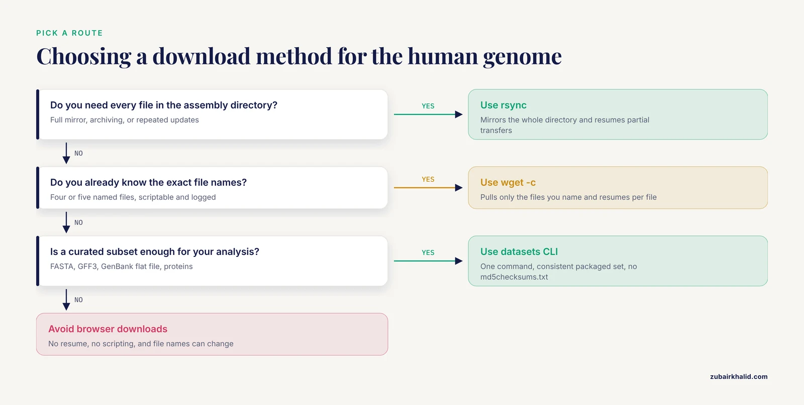
The walkthrough in the main guide presents three methods in sequence, but real projects require a decision, and the decision depends on what you plan to do with the files. Here is the honest tradeoff space.
| Method | What you get | Resumes after interruption | Gives complete assembly directory | Best for |
|---|---|---|---|---|
datasets CLI [1] | FASTA, GFF3, GenBank flat file, protein translations, packaged in a zip | Re-run the command and it re-downloads | No, curated subset only | First-time users, quick tests, scripts that want one command |
wget -c | Exactly the files you name | Yes, per file | No, unless you name every file | Pulling two or three known files over networks that block raw FTP |
rsync -avP | The entire assembly directory | Yes, including partial transfers | Yes | Mirrors, archiving, repeated updates |
| Browser download | Any single file | No | No | Grabbing one file interactively when writing commands is not worth it |
A few decision rules fall out of this table.
Use the datasets CLI when the zip contents match your needs. The tool wraps taxonomy, gene, and genome data behind one interface, and its recent updates have expanded programmatic access and tightened the connection between taxonomy queries and genome data [1]. If your analysis needs the FASTA and the GFF3 and nothing else, the one-command route is the shortest path and the least error prone, because the tool assembles a consistent set of files for you.
Use wget when you know the file names. Direct retrieval of four or five named files is transparent, easy to log, and trivially scriptable. Its weakness is completeness: nothing in a wget workflow tells you what you forgot to download. This is why the guide's walkthrough pairs wget with the file table in the main guide, and why the assembly_report.txt should always be on your list even if you never open it.
Use rsync when completeness or repeatability matters. A mirror of the full assembly directory captures files you did not know you would need later, such as the GenBank flat file directory or the CDS translations. Because rsync transfers only differences on subsequent runs, keeping the mirror current costs almost nothing after the first pull. The caution from the main guide bears repeating in decision form: never point rsync at the species level. The Homo_sapiens directory contains every human assembly ever deposited, and the result is measured in tens of terabytes.
Avoid the browser for anything automated. Browser downloads do not resume, cannot be scripted, and quietly change the file name if you download twice. They are fine for peeking at a directory listing, which is genuinely useful, but not for acquiring data.
One more consideration that rarely gets mentioned: provenance. For a publication or a clinical report, the question "exactly which genome files did you use?" must have a precise answer. A single rsync of one assembly directory answers it completely. A datasets zip answers it if you archive the zip alongside its dataset_catalog.json, which records what was inside. A pile of individually wget-ed files answers it only if you saved the command list. Whichever route you pick, archive the commands or the manifest with the data.
Worked Example: Building a Chromosomes-Only Primary FASTA
The complete FASTA contains roughly 640 sequences, and most of them are alt loci and scaffolds that fragment short-read alignments. Standard practice is to align against a reduced FASTA containing the assembled molecules, and the assembly_report.txt you downloaded is the authoritative source for identifying them. This section builds that reduced file step by step, without deleting anything you might need later.
Step 1: Look at the report structure.
head -n 40 GCF_000001405.40_GRCh38.p14_assembly_report.txtAfter several comment lines beginning with hash characters, you reach a tab-delimited table. The columns that matter here are Sequence-Name, Sequence-Role, RefSeq-Accn, and UCSC-style-name. Every row carries exactly one Sequence-Role, and the roles partition the whole assembly: assembled molecules (the chromosomes, including MT), unlocalized scaffolds, unplaced scaffolds, alt scaffolds, and a few special categories.
Step 2: Extract the RefSeq accessions for the assembled molecules.
awk -F '\t' '$2 == "assembled-molecule" {print $6}' \
  GCF_000001405.40_GRCh38.p14_assembly_report.txt > chr_accessions.txt
Column 2 is the sequence role and column 6 is the RefSeq accession. Inspect the result:
cat chr_accessions.txtYou should see the accessions for chromosomes 1 through 22, X, Y, and MT. If your downstream tools expect mitochondrial sequence under a particular identifier, confirm it appears here.
Step 3: Filter the FASTA by those accessions.
A two-pass awk reads the accession list first, then streams the FASTA, keeping only records whose header token matches:
awk 'NR==FNR { want[$1]=1; next }
     /^>/   { name=$1; sub(/^>/,"",name); keep=(name in want) }
     keep' chr_accessions.txt \
  GCF_000001405.40_GRCh38.p14_genomic.fna > GRCh38_primary.fna
The logic is worth understanding rather than copying blindly. When the current line is a FASTA header, the script strips the leading angle bracket and decides, based on membership in the wanted set, whether to keep this record and everything after it until the next header. Records not in the list are skipped entirely, so no sequence content leaks through.
Step 4: Index and verify the reduced file.
samtools faidx GRCh38_primary.fna
awk '{s+=$2} END {print s}' GRCh38_primary.fna.fai
grep -c '^>' GRCh38_primary.fna
The record count should now match the number of assembled molecules, and the summed length should equal the total length of the assembled molecules reported in assembly_stats.txt, not the full 3.34 gigabases of the complete FASTA. This distinction matters: the full total includes alt loci and scaffolds, so a mismatch between the two sums is expected and correct, not an error.
Keep the complete FASTA on disk even after building the primary-only file. If a later analysis concerns a region with an alt representation, such as the highly polymorphic major histocompatibility complex, you will want those alt sequences available, and re-downloading to get them is avoidable waste.
Worked Example: Converting Between RefSeq and UCSC Sequence Names
Sequence identifier mismatch is the quietest failure in genomics. A BED file of intervals named chr1 produces zero overlaps when intersected with a GFF whose seqids are NC_000001.11, and no tool raises an error, because both naming schemes are internally valid. The assembly_report.txt includes a UCSC-style-name column precisely to bridge the two conventions.
Build the mapping table:
awk -F '\t' '$8 != "na" && NR > 1 {print $6"\t"$8}' \
  GCF_000001405.40_GRCh38.p14_assembly_report.txt > refseq_to_ucsc.tsv
Column 6 is the RefSeq accession and column 8 is the UCSC-style name. The comparison filters out rows where no UCSC name exists, which the report marks with a placeholder, and skips header lines. Inspect it:
head refseq_to_ucsc.tsvEach line pairs a RefSeq accession with its browser-style equivalent, so NC_000001.11 maps to its chromosome 1 counterpart and alt scaffolds map to their alt-style names.
Rename FASTA headers in place, producing a new file:
awk 'NR==FNR { map[$1]=$2; next }
     /^>/   { name=$1; sub(/^>/,"",name);
              if (name in map) { sub("^>"name, ">"map[name]) } }
     { print }' refseq_to_ucsc.tsv \
  GCF_000001405.40_GRCh38.p14_genomic.fna > grch38_ucsc_named.fna
For every header, the script looks up the RefSeq token in the mapping table and rewrites the header before printing. Sequence content passes through untouched.
Rename the index accordingly. If you had already run samtools faidx on the original file, run it again on the renamed file. A .fai index is keyed on the header tokens, so an index built before renaming is silently wrong for the renamed file, and samtools faidx will usually rebuild or complain, but only if you let it.
Convert a BED file the same way:
awk 'NR==FNR { map[$1]=$2; next }
     { if ($1 in map) $1=map[name=$1]; print }' refseq_to_ucsc.tsv intervals.bed
A cleaner variant uses sed for the common case of chromosome-only files, but the awk approach generalizes to alt scaffolds, which is where naive sed substitutions typically mangle names.
The same logic applies in reverse if a collaborator sends UCSC-named data and your pipeline is RefSeq-native. Whichever direction you convert, convert once, at the boundary of your pipeline, and record the conversion in your methods. Converting ad hoc at multiple stages invites exactly the partial-mismatch errors this section exists to prevent.
Worked Example: Pulling a Specific Region with samtools faidx
Once the FASTA is indexed, extracting sequence for a gene, promoter, or variant window is a one-liner, and it is the fastest sanity check that your reference, your coordinates, and your expectations all agree.
The samtools faidx region syntax is accession:start-end, with coordinates in one-based, inclusive, closed form, matching how coordinates appear in GFF3 and in most variant catalogs. Suppose your region of interest sits on chromosome 8 and you have a pair of candidate coordinates from an annotation source. The illustration below uses round numbers chosen for readability; substitute your own:
samtools faidx GCF_000001405.40_GRCh38.p14_genomic.fna \
  NC_000008.11:145000000-145100000 > region.fa
Notes on behavior that surprise people:
- The accession must match the header token exactly.
samtools faidxkeys on the first whitespace-delimited token,NC_000008.11in this FASTA. A query forchr8fails, and a query forNC_000008without the version suffix fails, because the version is part of the token. Both failures are informative, not annoying: they confirm that you are not silently querying the wrong assembly. - Line wrapping does not matter. The index tracks byte offsets, so the extracted sequence is correctly joined regardless of how the FASTA is wrapped.
- Multiline region requests work. Provide several regions on the command line, or supply a file of regions with the batch mode of
samtools faidx, and each extraction lands in the output as its own record. This is the practical route for primer design, probe design, or pulling flanking sequence around a list of variants.
A useful cross-check couples extraction with your variant data. After calling variants against the reference you downloaded, extract a few hundred bases around a variant of interest, and compare the reference base at the variant position to the base reported in your variant call file. If they disagree, either your variant call coordinates are from a different assembly, or your reference is not the one you think it is. This five-minute check has caught more assembly-mismatch bugs than any log file.
For regions containing many ambiguous bases, remember that runs of N are legitimate reference content representing unsequenced or unresolvable gaps, and extracting through them yields Ns in your output. That is expected behavior, covered further in the misconceptions section below.
The Annotation Files: Working with the GFF3 and GenBank Flat File
The genome FASTA answers where the bases are; annotation answers what they mean. The assembly directory gives you two complementary annotation formats, and knowing when to reach for each prevents a lot of wasted parsing.
The GFF3 file, *_genomic.gff.gz, is the tab-delimited workhorse. Each feature occupies one line with nine columns: seqid, source, type, start, end, score, strand, phase, and attributes. Because it is line oriented, GFF3 is what awk, bedtools, and database loaders consume happily. The GenBank flat file, *_wgsmaster.gbff.gz, carries the same biology in a human-readable structured record, complete with provenance and feature qualifiers, and is what you want when you need to read context around a feature rather than intersect coordinates mechanically.
A first pass over the GFF3 establishes what it contains:
zcat GCF_000001405.40_GRCh38.p14_genomic.gff.gz | awk -F '\t' '$3=="gene"' | wc -lThe $3 column is the feature type, and counting gene lines gives you a headline number to compare against documentation or previous releases. Comment lines beginning with hash characters are skipped automatically by the awk filter because their field 3 is empty.
Extract gene records for one chromosome, with coordinates and gene names:
zcat GCF_000001405.40_GRCh38.p14_genomic.gff.gz \
  | awk -F '\t' '$1=="NC_000001.11" && $3=="gene" {print $4"\t"$5"\t"$9}'
Column 1 is the seqid, columns 4 and 5 are start and end, and column 9 carries the attributes including the gene name. This one-liner is the seed of many ad hoc analyses, from checking whether a candidate region contains annotated genes to building a gene-level summary of interval overlaps.
Check that annotation and FASTA agree on sequence identifiers. This is the single most valuable QC step for annotation files, and it takes three commands:
zcat GCF_000001405.40_GRCh38.p14_genomic.gff.gz \
  | awk -F '\t' '!/^#/ {print $1}' | sort -u > gff_seqids.txt
grep '^>' GCF_000001405.40_GRCh38.p14_genomic.fna \
  | sed 's/^>//' | awk '{print $1}' | sort -u > fasta_seqids.txt
comm -23 gff_seqids.txt fasta_seqids.txt
The comm command prints seqids present in the GFF but absent from the FASTA. Any output means the annotation references sequence your alignment index cannot resolve, and every downstream intersection involving those records will silently drop them. Because both files came from the same assembly directory, this check should produce no output, which is exactly the point: it confirms the pairing you assumed, and it will produce output the day a colleague hands you mismatched files.
Mind the coordinate conventions if you convert to BED. GFF3 coordinates are one-based and inclusive; BED coordinates are zero-based with an exclusive end. Converting naively by copying start and end into a BED shifts every interval by one base, which is invisible in casual inspection and ruinous for base-level analysis. If you convert, convert deliberately, and validate a handful of intervals against the FASTA with samtools faidx before trusting the conversion at scale.
Finally, the protein FASTA in the assembly directory pairs naturally with the GFF3: every protein record corresponds to a CDS feature, and the accessions link them. If your work touches protein-level questions, from functional annotation to the kind of variant-to-expression prioritization represented by projects combining variant catalogs with expression resources [7], having the translations locally avoids a second round of network queries later.
A Reusable Download Script with Error Handling
For anything you will run more than once, on more than one machine, or on behalf of collaborators, fold the walkthrough into a script that fails loudly instead of silently. The script below combines the download, verification, decompression, and indexing steps, and stops at the first failure rather than building downstream artifacts on bad data:
#!/usr/bin/env bash
set -euo pipefail

ACCESSION="GCF_000001405.40_GRCh38.p14"
BASE="https://ftp.ncbi.nlm.nih.gov/genomes/refseq/vertebrate_mammalian/Homo_sapiens/all_refseq/${ACCESSION}"
DEST="${HOME}/genomes/${ACCESSION}"

mkdir -p "${DEST}"
cd "${DEST}"

FILES=(
  "${ACCESSION}_genomic.fna.gz"
  "${ACCESSION}_genomic.gff.gz"
  "${ACCESSION}_assembly_report.txt"
  "${ACCESSION}_assembly_stats.txt"
)

for f in "${FILES[@]}"; do
  if [ ! -s "${f}" ]; then
    echo "Fetching ${f}"
    wget -c -t 5 -T 60 -q "${BASE}/${f}"
  fi
done

echo "Fetching checksum manifest"
wget -c -q "https://ftp.ncbi.nlm.nih.gov/genomes/refseq/vertebrate_mammalian/Homo_sapiens/all_refseq/md5checksums.txt"

echo "Verifying"
grep -F "${ACCESSION}" md5checksums.txt > local.md5
md5sum -c local.md5

echo "Decompressing and indexing"
gunzip -kf "${ACCESSION}_genomic.fna.gz"
samtools faidx "${ACCESSION}_genomic.fna"

echo "Cross-checking total length"
awk '{s+=$2} END {print s}' "${ACCESSION}_genomic.fna.fai"

echo "Done."
Design choices worth copying into your own scripts:
set -euo pipefailturns any failed command into a script exit. Without it, a failedwgetinside a loop sails onward and the verification step runs against whatever partial files exist, producing a confusing cascade of errors far from the root cause.- The
-sfile test skips files that already exist and are non-empty. Combined withwget -c, this makes the script safe to re-run: finished files cost nothing, interrupted files resume, and missing files download fresh. A script you can re-run fearlessly is a script you will actually run before every project. -t 5and-T 60on wget cap retries and set a network timeout, so a stalled connection fails fast and retries rather than hanging a pipeline overnight on a dead socket.gunzip -kfdecompresses while keeping the original archive. Keeping the compressed original preserves the byte stream that the MD5 manifest describes, which means you can re-verify the archive after any suspicion of trouble without re-downloading.- The length cross-check at the end reuses the technique from the main guide: summing the
.failengths and comparing, by eye or by assertion, to thetotal_sequence_lengthinassembly_stats.txtand to the figure reported by thedatasets summarycommand [1]. Two independent routes agreeing is stronger evidence than either alone.
To parameterize the script for other organisms or a future patch release, note that only the ACCESSION variable and the species directory path change. Resist the temptation to hardcode more than necessary, and resist equally the temptation to auto-discover the accession inside the script: a reference genome is something you choose deliberately and then record, not something a script should silently upgrade beneath an active analysis.
Verification Beyond Checksums: Building a Cross-Check Habit
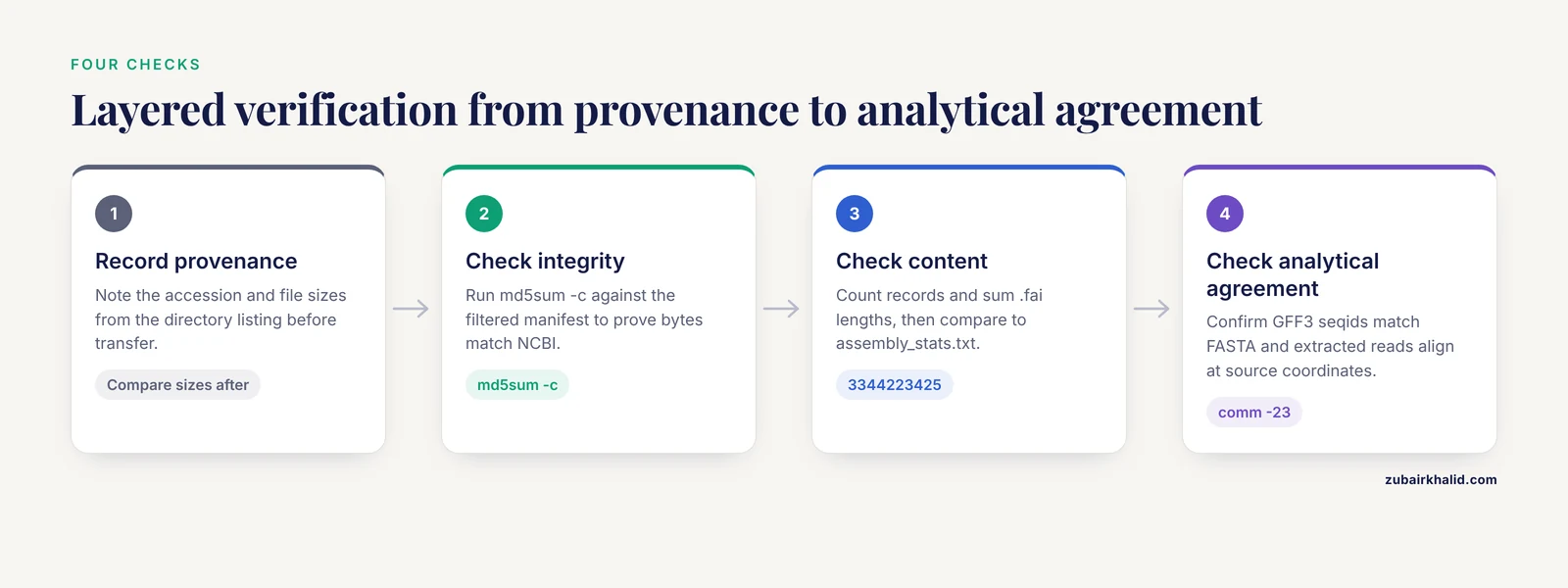
MD5 verification, covered in the main walkthrough, proves the bytes on your disk match the bytes NCBI published. It does not prove the file is the one your analysis expects, nor that your processing preserved it. A layered verification habit covers all three levels, and each layer costs seconds.
Layer 1: provenance. Before any transfer, record the accession and, ideally, the file sizes from the directory listing. After transfer, compare. A file whose size differs from the listing is incomplete before you even reach checksums. This is the fastest available check and catches the most common failure, a truncated transfer, immediately.
Layer 2: integrity. The md5sum -c step from the walkthrough. Filter the manifest to the files you actually downloaded, because the full manifest covers the entire human release and md5sum reports missing files as failures that are merely out of scope. On macOS without GNU coreutils, md5 -q prints the bare digest for one file, which you compare by eye or by script against the matching line of the manifest:
md5 -q GCF_000001405.40_GRCh38.p14_genomic.fna.gz
grep "genomic.fna.gz" md5checksums.txt
Layer 3: content. The record count and total length checks from the walkthrough, cross-referenced against assembly_stats.txt and the datasets summary. Content checks catch a subtler class of problem: the right file, fully transferred, processed wrongly. If you concatenated the FASTA with another file, or truncated it during an ill-advised text manipulation, checksums on the original archive still pass because you verified the archive, not your derived file. The derived-file checks catch that.
Layer 4: analytical agreement. The deepest check, and the one that pays for itself repeatedly: verify that independent artifacts agree with each other. The GFF3 seqid check from the annotation section above is one example. Another is extracting a region with samtools faidx and confirming the coordinate semantics behave as expected, one-based and inclusive, at the boundaries. A third is aligning a small set of known-good reads, or even a handful of sequences extracted from the reference itself, and confirming they align at their source coordinates. If reads extracted from chromosome 17 align to chromosome 17, your index, your naming, and your aligner invocation are all coherent.
The habit generalizes beyond this download to every large file you will ever pull from NCBI, from ClinVar releases distributed via FTP and programmatic tools [5] to annotation and assembly packages for other organisms. Layered verification is what turns "it downloaded successfully" from a hope into a statement you can defend in a methods section.
Downloading on Constrained Systems: WSL2, macOS, and Shared Clusters
The main guide notes that Windows users can run everything under WSL2, macOS users can substitute md5 -q, and both claims deserve the practical detail that makes them true in awkward environments.
WSL2. Install the tools through the distribution's package manager, for example on an Ubuntu-based distribution:
sudo apt update && sudo apt install wget curl rsync unzip md5samtoolscorrecting the last package name to your distribution's samtools package if the bundled name differs. Two environment-specific warnings matter. First, store the genome and its index on the Linux-native filesystem, under your home directory such as ~/genomes/, rather than under /mnt/c/, the mount point for Windows drives. Cross-filesystem I/O for the many small reads that indexing and alignment generate is dramatically slower, and this single placement decision often dominates total runtime. Second, disk space you see from WSL2 is the space of the Linux virtual disk, which can differ from what Windows reports; the df -h . check from step 1 of the walkthrough, run from inside WSL2 in the target directory, is the number that matters.
macOS. The core utilities differ in small, sharp ways. md5sum is absent, and md5 -q file prints the bare digest. GNU sed and BSD sed disagree on in-place editing flags, which affects any copied one-liner involving sed -i. The safest path is to install GNU coreutils and samtools through Homebrew, or to run everything inside a conda environment where the GNU toolchain is available consistently. The wget and rsync commands in the guide work natively, though macOS ships an older rsync; for the one-shot assembly mirror it behaves equivalently.
Shared clusters. Compute clusters usually provide wget, rsync, and samtools through their module system or as preinstalled binaries, and the conda route from the main guide works without administrator rights where module systems fall short. Two cluster-specific practices matter more than tool versions. First, download into scratch or project storage, not your home directory, because home quotas on shared systems are routinely smaller than the 10 to 15 GB budget this project needs once indexes and outputs accrue. Second, be a good cluster citizen: a download running for hours occupies little compute but holds a login node, and many clusters kill long login-node processes. If your cluster provides a dedicated transfer or data-mover node, use it; otherwise run the download inside a brief interactive job or detach it in a session manager so an accidental logout does not orphan it mid-transfer, then let wget -c or rsync -P resume.
In all three environments the same three principles apply: verify with the tools actually present on that system, keep data and indexes on the fastest local filesystem available to the analysis, and make every acquisition step re-runnable, because constrained systems fail more often, and resumption is the difference between a pause and a restart.
Download Speed and Parallel Fetching
The human FASTA is near 1 GB compressed, and the full assembly directory is larger. On a fast institutional connection a single stream saturates available bandwidth easily; on a typical residential connection the transfer takes minutes to tens of minutes, and on a congested one the resumable flags are what save you. A few techniques improve throughput without inviting trouble.
Fetch several files concurrently, modestly. The assembly directory contains multiple independent files, and downloading a few at a time overlaps the latency of each transfer:
printf '%s\n' \
  "${BASE}/GCF_000001405.40_GRCh38.p14_genomic.fna.gz" \
  "${BASE}/GCF_000001405.40_GRCh38.p14_genomic.gff.gz" \
  "${BASE}/GCF_000001405.40_GRCh38.p14_assembly_report.txt" \
  | xargs -n 1 -P 3 wget -c -q
Here -P 3 runs three wget processes at once, each still carrying -c so an interruption resumes cleanly. Keep the concurrency small. Hammering a public server with dozens of parallel connections is both discouraged and, past a modest number, unhelpful, because most clients are bandwidth limited rather than round-trip limited, and the marginal gain collapses while the burden on the shared service grows.
Single-file segmented downloaders exist, with a caveat. Tools that split one large file into ranged parallel segments can shorten wall-clock time on high-latency links, and their resume support is generally good. The caveat is operational: a segmented transfer produces the same final bytes but a more complicated failure mode, and you should only adopt one if you will still verify with md5sum -c afterward, which you should do regardless of tool. The verification step, not the download tool, is the actual guarantee.
Schedule large transfers for off hours. On shared institutional networks, transfer speed at two in the morning routinely differs from speed at two in the afternoon by a factor that matters more than any tooling choice. Since the download is fully scriptable and resumable, running it overnight inside a session that survives logout is usually the cheapest speed improvement available.
Do not re-download what you already have. Every method in this guide supports resumption or idempotent re-running, and the re-runnable script in the earlier section skips completed files outright. The largest speed improvement available to most people is simply never restarting a transfer that already finished.
Finally, set expectations honestly for the steps after download. Decompression and samtools faidx indexing take minutes; bwa index or a minimap2 index build takes tens of minutes and considerable memory on a typical workstation, as the main guide notes. Optimizing the five-minute download while under-provisioning the hour-long index build optimizes the wrong bottleneck.
Keeping a Local Mirror Current Without Breaking Pipelines
Reference genomes change slowly but not never, and the patch cycle of GRCh38 means a mirror maintained across months will eventually fall behind. The challenge is updating without invalidating the analyses that depend on the old files, and the solution is separation: mirror updates happen when you choose, pipeline version pinning happens once, and the two never interact accidentally.
Update on your schedule with rsync. Re-running the rsync command from the walkthrough transfers only files that changed or appeared since the last run. For a patch release, NCBI publishes the new assembly under its own accession directory, so your existing directory remains byte-identical and a new sibling directory appears. This design is a gift: updates are purely additive at the directory level, and nothing you built against the old directory is touched. Scheduling the rsync, for example from a monthly cron entry, keeps the mirror current while leaving every historical release intact.
Pin, do not float. Every pipeline should reference a full accession such as GCF_000001405.40, never the phrase "the current human reference." The distinction matters because RefSeq re-releases its packaging with each GRC patch, so "current" is a moving target while the accession is a fixed address. Record the accession, the file sizes, and the checksum status in a small manifest alongside the data:
{ echo "assembly: GCF_000001405.40 GRCh38.p14"
  echo "downloaded: $(date -I)"
  md5sum GCF_000001405.40_GRCh38.p14_genomic.fna.gz
} > MANIFEST.txt
This manifest costs seconds to produce and answers the version question definitively in any review, audit, or debugging session months later.
Re-verify after updates, not just after initial download. The md5sum -c step belongs in your update routine too, not because NCBI data is unreliable but because your storage is not. Silent bit rot on large archives is rare but real, and a checksum sweep before rebuilding an index is cheap insurance against an afternoon of mysterious aligner failures.
Decide deliberately when to rebuild indexes. Because patch releases leave primary chromosome sequence stable, a new patch rarely forces an index rebuild, as the main guide's mistakes section explains. The trigger for rebuilding is a change that affects your analysis: a patch that alters primary sequence in your regions of interest, a change in the alt loci you align against, or a deliberate migration to a new major assembly. Diffing assembly_stats.txt between the old and new releases is the fastest way to see whether anything you care about changed, and if the totals and the sequences you use are unchanged, the rational choice is to keep the existing index.
Archived releases remain available. Older assemblies, including GRCh37-era RefSeq packaging, stay on the FTP tree in their own directories, so legacy projects can re-fetch their exact reference years later. This is another argument for recording the accession: it is the key that unlocks the identical file a decade from now, which is what "reproducible" means in practice.
Common Misconceptions About the Human Reference Genome
The main guide catalogs operational mistakes. This section addresses beliefs that are wrong in a quieter way, because they shape how people interpret results even when every command ran perfectly.
"The reference genome is one person's genome." It is not. The reference is a haploid mosaic assembled from multiple sources, and no individual carries it. This has direct consequences: a diploid sample aligned against a haploid reference produces heterozygous sites as one allele matching the reference and one not, and copy-number and structural variant interpretation inherits the reference's specific representation of duplicated regions. Fully phased diploid assemblies, now achievable with modern sequencing, resolve structural variants with a clarity the standard reference cannot match precisely because they do not force every locus through a single mosaic [8]. When your question touches structural variation or population diversity, treat the reference as a coordinate frame, not as a truth about human genomes.
"Runs of N mean the download is corrupt." The reference contains long stretches of Ns representing gaps and unresolvable sequence. Their presence is expected content, not corruption, and the length cross-check distinguishes the two cases cleanly: corrupt files fail checksums or produce a length mismatch, while intact files contain the same Ns the published release contains. The GRC continues working to replace missing sequence, and material long characterized cytogenetically, including certain satellite and heterochromatic sequences, remains incompletely represented in the reference and in the browsers built on it [3]. Ns in the current release are a map of what remains unresolved, which is itself useful information.
"hg38 and GRCh38 are different assemblies." They are the same underlying GRC assembly packaged by different institutions, with UCSC adding its own naming convention and, in some releases, extra sequences. What differs, and matters, is sequence naming and occasionally the exact set of included contigs. The UCSC-style-name column in assembly_report.txt exists precisely because both representations circulate, and the browser landscape of UCSC, Ensembl, and NCBI is the main source of the naming confusion in the first place [3]. The worked conversion example earlier in this guide handles the naming; the habit to build is asking, for every external file you receive, "which packaging and which naming convention?"
"Downloading the FASTA gives me an annotated genome." The FASTA is bare sequence. Annotation arrives separately, in the GFF3 or GenBank flat file, and only the pairing of a specific FASTA with its matching annotation from the same assembly directory is guaranteed coherent. The seqid cross-check described in the annotation section is how you confirm the pairing when files come from different hands.
"The datasets CLI replaces the FTP site." They are complementary, not competing. The CLI offers curated, convenient access to genomes, genes, and taxonomy with programmatic tooling behind it [1]; the FTP tree offers the complete, file-level view of every release with resumable mirroring. Pipelines that grow usually start at the CLI and grow into the FTP tree, and knowing both means neither growth requires a scramble.
"A k-mer index of the whole genome is the only way to search it." Full indexes are the default, but the size and query-time tradeoffs of exhaustive k-mer indexes have been studied directly on the human genome, and sampling strategies reduce both index size and query cost for some search workloads [4]. The practical lesson is not that one approach is universally right, but that index construction is a design decision with measurable consequences, worth matching to the question rather than defaulting blindly.
Troubleshooting Quick Reference
The failures below account for the overwhelming majority of trouble reported with this download. Each row pairs the symptom you observe with the cause and the fix.
| Symptom | Likely cause | Fix |
|---|---|---|
wget returns a 404 | Accession or file name wrong for the current release; or a patch superseded the one in your notes | Confirm the live accession with the datasets summary command [1]; list the directory over HTTPS in a browser; correct the variable in your script |
| Transfer stalls at a fraction of the size and times out | Network interruption or firewall idle-timeout | Re-run with wget -c; the transfer resumes rather than restarts |
md5sum -c prints FAILED for one file | Truncated or corrupted transfer | Delete that file, re-run the download with -c, re-verify; if it fails again, switch to rsync -P, which detects and repairs partial transfers natively |
gunzip reports unexpected end of file | The archive is incomplete despite a plausible-looking size | Same as the checksum failure path; never debug a truncated archive, replace it |
samtools faidx reports a missing or malformed line | The .fai is stale relative to the FASTA, often after renaming headers | Delete the .fai and regenerate it against the current FASTA |
grep -c '^>' returns a number far from the expected range | You decompressed a different or older file, or concatenated files accidentally | Re-check which file you indexed; re-run the checksum verification; compare the .fai length sum to assembly_stats.txt |
| Alignment runs but every read maps oddly or nowhere | Index built from a different file than the one reads assume, or assembly mismatch between read prep and reference | Confirm the accession on the indexed FASTA; confirm the coordinate system of any accompanying intervals; rebuild the index if the FASTA changed |
| BED intervals produce zero overlaps with the GFF | Sequence naming mismatch, chr-style versus accession-style | Build the mapping from assembly_report.txt and convert once at the pipeline boundary, as in the worked example above |
No space left on device during indexing | Disk filled by FASTA plus index plus earlier outputs | Free space or relocate; re-run the idempotent script, which skips completed steps |
datasets download produces a zip that fails to unzip | Interrupted CLI download | Delete the zip and re-run the command; the tool re-fetches cleanly |
| FTP connection refused or blocked outright | Institutional firewall blocking the FTP protocol | Switch the URL prefix to HTTPS, which serves identical content and passes most firewalls |
Two meta-rules shorten every debugging session. First, when a failure appears hours after download, suspect the download before the analysis, and spend the sixty seconds on verification before reading aligner logs; this ordering resolves most mysteries immediately. Second, when a mismatch appears between two files, suspect their assembly versions before their contents, because different-version pairing is by far the most common way two individually correct files fail together.
Putting It to Work: Downstream Uses of a Verified Reference
A verified, indexed reference is not an end point; it is the substrate every serious analysis stands on. Seeing where it plugs in clarifies why the verification discipline above is worth the seconds it costs.
Cohort sequencing QC. Quality control pipelines for whole-genome and whole-exome cohorts align raw reads against the reference before computing coverage, contamination, and call-rate metrics, and scalable frameworks designed for cohorts of hundreds of thousands of samples assume a properly indexed reference as their first dependency [9]. Every downstream metric in such pipelines inherits the identity of the reference, which is why the manifest habit matters: when a QC outlier traces back to reference identity, the manifest turns a day of archaeology into a one-line answer.
Variant annotation with ClinVar. ClinVar, the public archive of human genetic variants and their clinical interpretations, distributes its complete data via FTP and programmatic interfaces [5]. Variant calls made against the reference you downloaded share its coordinate system, so annotating called variants against ClinVar is a direct coordinate intersection with no lifting step. The prerequisite is the one this guide enforces throughout: your call coordinates and the ClinVar release must describe the same assembly, and the accession in your manifest is how you confirm it.
Copy-number and structural analysis. CNV callers interpret read depth against the reference, and benchmarking against curated variant catalogs is standard practice in that space [6]. Because depth-based methods are sensitive to the reference's representation of duplications and gaps, the regions-of-caution caveat from the misconceptions section applies with extra force here, and the alt-loci decision from the walkthrough shapes results directly.
Expression and variant prioritization. Work that connects variant catalogs to tissue-level expression, in the spirit of projects combining variant resources with expression data such as GTEx, prioritizes mutations in commonly expressed proteins [7]. The chain runs through the same reference: aligned reads, called variants, matched coordinates, then expression context. A reference verified at acquisition time keeps every link of that chain trustworthy.
Reference-aware method development. Even methodological work, such as evaluating index structures for sequence search, benchmarks against the human genome specifically because its size and repetitiveness stress the method [4]. Having the reference locally, verified and indexed, is what makes such evaluation reproducible by others who download the same accession.
Phased and pangenome-adjacent work. As phased diploid assemblies become routine, comparisons against the standard reference remain the common coordinate frame for reporting, even when the analysis itself goes beyond the reference [8]. The download this guide covers is therefore not superseded by newer assembly styles; it remains the shared canvas on which they are compared.
The unifying theme is that every one of these applications depends on a chain of identity: this FASTA, this accession, this checksum, this index. Establishing that chain once, on the day you download, is the small investment that every downstream week draws on.
Frequently Asked Questions
Which file on NCBI FTP is the actual human genome sequence?
The file GCF_000001405.40_GRCh38.p14_genomic.fna.gz in the directory genomes/refseq/vertebrate_mammalian/Homo_sapiens/all_refseq/GCF_000001405.40_GRCh38.p14/ is the complete genome sequence in FASTA format. It contains all chromosomes, unplaced and unlocalized scaffolds, and alternate loci, totaling about 3.34 gigabases.
What is the difference between GCF and GCA accessions?
GCF accessions are RefSeq records curated by NCBI staff, while GCA accessions are the original GenBank submissions from the assembly's producers. For the human reference, GCF_000001405 is the RefSeq version of GRCh38 and is the one most pipelines and annotation resources expect.
How large is the human genome download?
The compressed genome FASTA is roughly 1 GB and decompresses to a little over 3 GB. With annotation files, protein translations, and an alignment index, budget around 10 to 15 GB of disk space for a working setup.
Should I use FTP, rsync, or the datasets CLI?
Use the datasets CLI when you want the FASTA plus standard annotation quickly with one command. Use wget with -c for specific files over networks that block raw FTP. Use rsync when you want the complete assembly directory or plan to keep a mirror updated.
How do I download GRCh37 instead of the current assembly?
GRCh37 lives on the same FTP tree under its own assembly directories, and archived RefSeq releases remain available. You can also list available human assemblies with datasets summary genome taxon "Homo sapiens" without the -reference flag and locate the older accession from the results.
Why does the FASTA contain more than 25 sequences?
Beyond chromosomes 1 through 22, X, Y, and M, the file includes unlocalized and unplaced scaffolds, alternate loci for regions of high structural diversity, and patch sequences. The assembly_report.txt file classifies every sequence so you can filter or rename them as needed.
How do I confirm the download is complete and undamaged?
Run md5sum -c against the filtered lines of md5checksums.txt, then sum the sequence lengths in the .fai index and compare the total to the total_sequence_length in assembly_stats.txt. Both checks passing means the file is intact and complete.
How often does the human reference genome change?
The GRC releases patches to GRCh38 periodically and major assemblies far less often, and RefSeq re-releases its GCF packaging with each patch. Check the current accession with datasets summary genome taxon "Homo sapiens", reference before starting a new project rather than assuming a version from memory.
Sources
- NCBI taxonomy: enhanced access via NCBI datasets.
- Introducing RefSeq and LocusLink: curated human genome resources at the NCBI.
- About classical molecular genetics, cytogenetic and molecular cytogenetic data not considered by Genome Reference Consortium and thus not included in genome browsers like UCSC, Ensembl or NCBI
- The effects of sampling on the efficiency and accuracy of k-mer indexes: Theoretical and empirical comparisons using the human genome
- ClinVar: improvements to accessing data.
- B-229 Benchmarking of Bioinformatics and Molecular Tools for Copy Number Variants Calling From Human Genome: A Detailed Look on Single Exons
- GTExome: Modeling commonly expressed missense mutations in the human genome
- Fully Phased Sequence of a Diploid Human Genome Determined de Novo from the DNA of a Single Individual
- WxS-QC - a quality control pipeline for human Whole-Genome and Whole Exome sequencing cohorts