Why Does DESeq2 Throw 'Model Matrix Not Full Rank'?
By Dr. Zubair Khalid, DVM, MS, PhD ·

The single most common cause of the "model matrix not full rank" error in DESeq2 is perfect confounding between two columns of your sample metadata, and the most frequent version of that problem is a batch variable that lines up exactly with the condition of interest. Every treated sample was sequenced on Tuesday and every control sample on Wednesday, so the design formula ~ batch + condition asks DESeq2 to estimate two effects that cannot be separated from each other. The second most common cause is accidentally including a metadata column that has a unique value for every sample, such as a sample ID, library name, or patient identifier, which makes the design matrix mathematically impossible to fit.
The first thing to check takes about thirty seconds. Cross-tabulate the factors in your design with table() and then compute the rank of the design matrix exactly as DESeq2 will build it:
with(coldata, table(batch, condition))

mm <- model.matrix(~ batch + condition, data = coldata)
qr(mm)$rank == ncol(mm)
If table() shows a block-diagonal pattern, with counts sitting on the diagonal and zeros everywhere else, the two factors are perfectly confounded and no statistical tool can estimate them separately. If qr(mm)$rank is smaller than ncol(mm), the matrix is rank deficient and DESeq2 will refuse the design. This article explains why the error happens, walks through the causes from most common to rarest, gives you a diagnostic sequence you can run in five minutes, and shows how to fix the design so the analysis stays valid.
What the Error Actually Means
DESeq2 models raw count data with a generalized linear model (GLM), a regression framework in which the expected count for each gene is written as a linear combination of an intercept and the columns of a design matrix. The design matrix, sometimes called the model matrix, has one row per sample and one column per estimable parameter, including the intercept and one column for each non-baseline level of each factor. DESeq2 builds this matrix from the design formula and the sample metadata table (colData) using the same model.matrix() function you would call by hand.
Rank is the number of independent columns in a matrix. A matrix is full rank when no column can be written as a weighted sum of the other columns. The GLM can only estimate a coefficient for each independent direction in the matrix. When a column is redundant, the coefficients are not identifiable, meaning infinitely many coefficient values fit the data equally well and no unique answer exists. In that situation the design matrix has a rank smaller than its number of columns, which is exactly what "not full rank" reports.
A concrete example makes this clear. Suppose you have six samples, three treated and three control, and the treated samples were all prepared in batch B while the controls were all prepared in batch A. The design matrix for ~ batch + condition contains an intercept, a batch column, and a condition column. The batch column and the condition column are identical up to a sign flip, because knowing a sample's batch tells you its condition perfectly. The matrix has three columns but a rank of only two. DESeq2 detects this before fitting and stops with the error rather than silently dropping a coefficient and reporting results whose meaning depends on an arbitrary choice.
Why DESeq2 Stops Instead of Guessing
DESeq2 runs an explicit rank check when you create the dataset object. The DESeqDataSetFromMatrix() function takes an argument checkFullRank, which defaults to TRUE when the design is not a single factor with no intercept, and it throws the error at object construction time rather than during fitting. This early failure is deliberate. Fitting a rank-deficient GLM in R does not always fail loudly. Base R's lm() fits such models, marks the redundant coefficients as NA, and reports aliased terms through alias(). A count model fitted this way would return log2 fold changes for some coefficients that depend entirely on which redundant column the software happened to drop.
Silent coefficient dropping is dangerous in differential expression because the dropped term is usually the one you care about. If batch and condition are confounded and the software drops the condition column, every apparent treatment effect is indistinguishable from a batch effect and the reported fold changes describe the confound, not the biology. Refusing to run is the correct behavior, even though the error message is terse and gives no hint about which column is the problem.
It also matters that the error fires before dispersion estimation and shrinkage. Published DESeq2 workflows across many domains, from multi-site human fibroblast comparisons [1] to GLA-edited podocyte models of Fabry disease [2] and four-group Ang II stimulation designs in smooth muscle cells [3], depend on the coefficient structure being estimable. A design matrix that passes the rank check produces coefficients whose meaning matches the design formula. A rank-deficient one would produce coefficients whose meaning is undefined, and the downstream gene lists, pathway enrichments, and rankings built on them would inherit that ambiguity. The same concern about model assumptions propagating into downstream interpretation applies to gene-set analysis more broadly, where careless statistical choices have been shown to distort results substantially [4].
The Causes Ranked From Most to Least Common
The error has a short list of underlying mechanisms. In practice, nearly every occurrence falls into one of the following seven categories. Read them in order, because the first two account for the large majority of cases in real RNA-seq projects.
1. Batch Perfectly Confounded With the Condition of Interest
This is the classic version of the error and the reason most people encounter it. Batch effects are technical differences introduced by processing samples in separate groups, such as different library preparation dates, different sequencer flow cells, different operators, or different library preparation kits. When the batching scheme tracks the experimental condition exactly, condition and batch are two names for the same split in the data.
The failure looks like this. You plan ~ batch + condition because you have read that DESeq2 can adjust for batch. You build the dataset:
dds <- DESeqDataSetFromMatrix(
  countData = cts,
  colData   = coldata,
  design    = ~ batch + condition
)
# Error in DESeqDataSetFromMatrix :
#   The design matrix contains 0 non-zero rows... (or)
#   model matrix not full rank!
Wait, the exact wording you will see is straightforward: the error names the model matrix and stops construction. The confirmation step is the cross-tabulation:
with(coldata, table(batch, condition))
#         condition
# batch    control treated
#   batch1       3       0
#   batch2       0       3
Zeros on the off-diagonal mean perfect confounding. There is no fix that recovers the treatment effect from this experiment, because the experiment never contained the information needed to separate biology from batch. The honest options are to report the analysis as a confounded comparison of combined batch-and-condition groups, or to re-run the experiment with balanced batching. Publishing such an analysis without acknowledging the confound is a recognized pitfall in the differential expression literature, and tool comparison work on bulk RNA-seq projects emphasizes that design quality sets a ceiling on what any downstream method can recover [5].
If the confounding is partial rather than perfect, meaning some batches contain samples from both conditions, the design can remain full rank. Partial confounding inflates uncertainty in the coefficients but does not make them unidentifiable. The cross-tabulation distinguishes the two situations immediately, which is why it is the first diagnostic step.
2. A Metadata Column With One Level Per Sample
The second most common cause is including a column whose value is unique for every sample. Sample names, library IDs, patient IDs when each patient contributed exactly one sample, sequencing lane assignments when each library occupied its own lane, and file names all have this property. A factor with as many levels as samples contributes one indicator column per level, which perfectly spans the data and leaves no residual degrees of freedom for anything else.
The mechanism is worth understanding because it produces the same error from innocuous-looking metadata. Suppose you merge two metadata tables and accidentally carry along a sample_id column, then write:
design(dds) <- ~ sample_id + conditionWith six samples and six distinct sample_id levels, the design matrix has an intercept, six sample indicator columns, and a condition column, and the condition column is a linear combination of the sample indicators. The rank equals the number of samples, which is less than the number of columns, and the check fails.
The rule to internalize: a blocking factor is only useful in a DESeq2 design when samples are repeated within its levels. A patient identifier earns its place in the formula when each patient provides both a treated and a control sample, as in matched tumor and non-tumor comparisons of the kind performed in TCGA cholangiocarcinoma analyses [6]. The same identifier is a rank killer when each patient contributed a single sample.
3. A Covariate That Is a Linear Combination of Other Columns
Rank deficiency does not require two factors to be confounded. Any column that can be written as a weighted sum of the others breaks the rank. Three patterns cover most cases:
- A total column included alongside its components, for example
cell_count_totaltogether withcell_count_liveandcell_count_dead. - Percentage columns that sum to 100 across categories, such as including all four cell-type fraction estimates from a deconvolution tool alongside an intercept.
- A numeric covariate duplicated at a different scale, such as including both weight in grams and weight in kilograms.
These are sneakier than factor confounding because the columns look independent in the cross-tabulation, which shows counts rather than collinearity. The diagnostic is numeric, and the fix is simply to drop one member of each redundant set, usually the derived total or the last percentage category.
4. Nested Designs With Empty Cells
Hierarchical designs, where donors contain cell lines or litters contain pups, fail full rank when the nesting is incomplete. If you write ~ donor + cell_line but some cell lines were derived from donors that contributed no other cell lines, the donor indicators and the cell line indicators overlap in ways that leave columns aliased. The correct construction is usually a single combined grouping variable:
coldata$donor_cellline <- paste(coldata$donor, coldata$cell_line, sep = "_")
design <- ~ donor_cellline + condition
This collapses the hierarchy into one blocking factor whose levels are the actual independent units. Multi-donor human tissue studies face exactly this structural question. In the fibroblast study cited above, seven primary cell lines from different anatomic sites were profiled, and hierarchical clustering grouped samples by anatomic site of origin rather than by donor, with sex and age effects reported as negligible [1]. That pattern is a reminder to check which metadata axis actually drives the variance before deciding what belongs in the design formula, because a blocking factor that does not correspond to real structure in the data can consume degrees of freedom without buying you anything.
5. Interaction Terms With Unobserved Combinations
Interaction terms multiply the columns of two factors, creating one column per combination of their levels. Every combination present in the interaction must be populated by at least one sample, and in practice you want several per cell. If you specify ~ genotype + treatment + genotype:treatment but one genotype was never exposed to one treatment, the corresponding interaction column is all zeros and the matrix loses rank.
Factorial designs with complete cells are the standard for interaction testing, and they are common in the applied DESeq2 literature. The Ang II smooth muscle cell study cited above used four groups, negative control, siDKK1 knockdown, negative control with Ang II, and siDKK1 with Ang II [3], which is a textbook two-by-two factorial. That design supports a full-rank model with main effects and an interaction only because all four cells were populated. Remove any one cell and the interaction term breaks the rank check. The CTVT vincristine response study illustrates the multi-group case, with ten tumors split across complete response, partial response, and resistance categories [7]. A response factor with three levels needs every level represented, and a design that also tries to add a second factor crossed with response will fail if any response-by-factor combination is empty.
6. Metadata Assembly Mistakes
Some rank errors are not design errors at all but data handling errors that make the design look confounded when the real experiment was fine:
- Row misalignment. If the row order of colData does not match the column order of the count matrix, DESeq2 will attempt to match by names, and any mismatch can pair samples with the wrong metadata. A
batchcolumn that was correct in the spreadsheet becomes nonsense after a silent sort in a previous script. Verify alignment withidentical(colnames(cts), rownames(coldata))before building the dataset. - Whitespace and case inconsistencies. "Batch1" and " batch1" are different factor levels in R. A trailing space can split one batch into two, creating an apparent one-sample-per-level column and a rank failure. Run
levels(factor(coldata$batch))and inspect the output for near-duplicates. - Stale factor levels. If you filtered samples out of colData but the columns kept unused levels, factors retain empty levels that add all-zero columns to the design matrix. Fix this with
droplevels(coldata)on every factor, or globally withcoldata[] <- lapply(coldata, function(x) if (is.factor(x)) droplevels(x) else x). - Numeric covariates read as characters. Age imported as a character column and converted to a factor generates one level per distinct age string, which in small studies approaches one level per sample.
These are unglamorous causes, but they are frequent, and they explain why the same design formula works on a colleague's machine and fails on yours.
7. Rare Numeric and Structural Edge Cases
A few unusual situations produce the error. A continuous covariate that is constant across all samples, which happens when a column was filled in only for a subset of samples and the remainder got a default value, contributes a column indistinguishable from the intercept. A continuous covariate recorded at only two distinct values is statistically identical to a two-level factor, which is not itself an error but becomes one when combined with other structure. Finally, designs written with explicit removal of the intercept, using a formula like ~ 0 + group, behave differently in model.matrix(), and combining a no-intercept parameterization with additional factors can create aliased full-dummy sets that fail the check.
Troubleshooting Table
The table below maps the symptoms you observe to the most likely cause, a fast confirmation step, and the fix.
| Symptom | Likely cause | How to confirm | Fix |
|---|---|---|---|
Error appears with ~ batch + condition, and every batch contains only one condition | Perfect confounding of batch and condition | table(batch, condition) shows zeros off the diagonal | Redesign is required, or model the combined grouping and report the confound |
| Error appears after adding a metadata column to the design | Column has one level per sample | length(levels(factor(col))) == ncol(cts) | Remove the column from the design unless samples repeat within its levels |
| Error appears with several numeric covariates | Linear combination among columns | caret::findLinearCombos(mm) names the columns | Drop the redundant total, percentage, or rescaled column |
Error appears with ~ donor + subtype or similar | Nested or incomplete blocking structure | Cross-tabulation shows donors unique to subtypes | Combine into one grouping variable, ~ donor_subtype + condition |
Error appears with genotype:treatment in the formula | Empty cell in the factorial | table(genotype, treatment) has a zero cell | Drop the interaction, add the missing samples, or collapse levels |
| Error appears on one machine but not another | Metadata misalignment or stale factor levels | identical(colnames(cts), rownames(coldata)), levels() inspection | Re-align metadata by names, droplevels() all factors |
| Error appears with a continuous covariate | Constant or near-constant column | length(unique(na.omit(col))) == 1 | Drop the column or fix the missing values it was masking |
Coefficients are NA in a limma or lm fit with the same design | Aliased columns confirmed independently | alias(lm(y ~ ., data = mm)) | Same fixes as above, the rank problem predates DESeq2 |
A Five-Step Diagnostic Sequence
Run these five steps in order whenever the error appears. The whole sequence takes minutes and identifies the specific offending columns rather than just confirming that something is wrong.
Step 1. Verify metadata alignment. Confirm that the metadata rows describe the count matrix columns in the right order.
identical(colnames(cts), rownames(coldata))
setdiff(colnames(cts), rownames(coldata))
If the first call returns FALSE, fix the metadata table before touching the design. Many apparent rank errors disappear once the metadata actually describes the samples.
Step 2. Cross-tabulate every pair of design factors. For each pair of variables in the formula, print the contingency table and look for zero cells and block-diagonal structure.
with(coldata, table(batch, condition))
with(coldata, table(donor, condition))
with(coldata, table(genotype, treatment))
Zero off-diagonal cells mean perfect confounding. Zero cells anywhere in a crossed pair predict interaction failures. Also check each single factor for levels with only one sample, since singleton levels are frequent contributors.
Step 3. Build the matrix and measure the rank. Reconstruct the exact matrix DESeq2 will use and compare its rank to its width.
mm <- model.matrix(~ batch + condition, data = coldata)
c(rank = qr(mm)$rank, ncol = ncol(mm))
A gap between the two numbers confirms rank deficiency and tells you how many columns are redundant. The limma package provides the equivalent check as limma::is.fullrank(mm), which returns TRUE or FALSE and, in the failure case, identifies the responsible columns through limma::nonEstimable(mm).
Step 4. Name the linear dependencies. The caret package computes the explicit linear combinations that reduce the rank, which turns an abstract error into a concrete list of columns to drop.
caret::findLinearCombos(mm)The output lists the column indices involved in each dependency and the coefficients of the combination. A dependency like batchB = intercept - batchA tells you the batch columns are redundant with the intercept structure, and combined with the cross-tabulation from Step 2 you will know whether the root cause is confounding or over-parameterization.
Step 5. Confirm the fix restores full rank. After adjusting the design, repeat Step 3 before recreating the DESeqDataSet.
mm2 <- model.matrix(~ condition, data = coldata)
qr(mm2)$rank == ncol(mm2)
Only when this returns TRUE should you rebuild the dataset and proceed to DESeq().
Two exploratory checks belong alongside these steps because they prevent the opposite mistake, which is fixing the rank error in a way that ignores real structure in the data. Principal component analysis on variance-stabilized counts shows which metadata axis dominates the sample distances, and published analyses routinely run PCA before testing, as in the Fabry podocyte study [2] and the clear cell renal carcinoma workflow that paired DESeq2 differential expression with PCA [8]. The fibroblast site-versus-donor finding [1] is a good model for the habit of examining clustering patterns before committing to a design. If PCA says tissue site explains most of the variance, a design that pretends otherwise will produce results nobody can interpret.
How to Fix the Design Without Breaking the Analysis
The right fix depends on the cause. The wrong fix, which is tempting in every case, is to delete columns from the formula until the error goes away and then report the results as if the change were neutral. Each fix below preserves the scientific question while restoring estimability.
Drop the Confounded Covariate and Report the Limitation
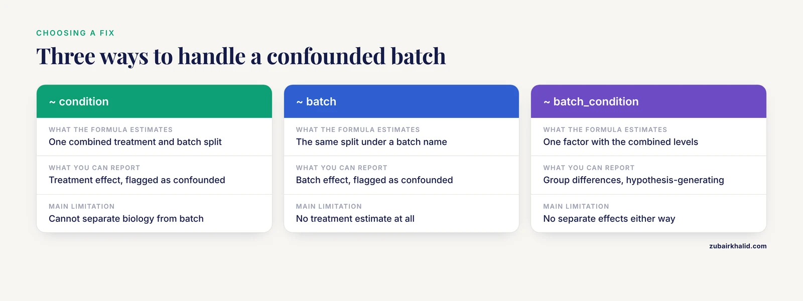
When batch and condition are perfectly confounded, the only full-rank designs are ~ condition alone, ~ batch alone, or a combined factor ~ batch_condition. All three model the same split in the data under different names. Run ~ condition, state in the results that treatment and batch are confounded and that treatment effects cannot be separated from batch effects, and treat the gene list as hypothesis-generating. This is not a workaround to hide. Confounded designs are a known structural weakness in RNA-seq projects, and honest limitation reporting is part of the quality assessment that differential expression work increasingly emphasizes [5].
Use Blocking Factors Correctly for Paired Designs
When the confounding structure is actually repeated measurement, blocking is the right tool rather than the problem. In a paired experiment where each donor contributes both a treated and a control sample, ~ donor + condition is full rank and estimates the treatment effect within donors, which is exactly what you want. Matched tumor and normal comparisons of the kind performed on TCGA cohorts [6] fit this pattern. The requirement is balance: every level of the blocking factor must contain samples from more than one condition. If some donors contributed only treated samples and others only controls, the blocking factor and the condition are partially or fully confounded and you are back in the Step 2 cross-tabulation.
Combine Nested Factors Into a Single Grouping Variable
For hierarchical designs, replace the separate factors with their interaction as a single factor. This preserves the between-unit blocking while removing the aliasing:
coldata$unit <- interaction(coldata$donor, coldata$cell_line)
design <- ~ unit + condition
This construction also handles the common case where a covariate such as sex or age is recorded at the donor level and would otherwise be redundant with donor indicators.
Drop One Member of Each Redundant Numeric Set
For collinear numeric covariates, keep the interpretable one. Keep component counts and drop the total, keep all-but-one category of a percentage set, keep one scaling of a duplicated measurement. Re-run findLinearCombos() after each removal until it reports no combinations.
Repair the Metadata Instead of the Formula
When the cause is misalignment, whitespace, or stale levels, the design formula was correct all along. Fix the metadata table, run droplevels(), verify with Step 3, and rebuild. Resist the urge to change the formula in this scenario, because the original formula was answering the right question.
Know When DESeq2 Is the Wrong Tool
DESeq2's design formulas handle fixed effects only. There is no random effects term, so designs with crossed random factors, deeply unbalanced repeated measures, or many hierarchical levels exceed what the formula syntax can express. Two alternatives cover this ground. The limma-voom pipeline supports within-block correlation through duplicateCorrelation for repeated measures, and comparative assessments of differential expression methods for bulk RNA-seq report meaningful performance differences between GLM-based edgeR, limma-based, and DESeq-family approaches depending on the comparison structure [5]. Mixed model frameworks in the general statistical literature, of the kind used for diet response modeling in animal studies where diet enters as a fixed effect alongside other model terms [9], provide the conceptual template that linear mixed model tools for RNA-seq implement directly. Moving tools is a real decision with real trade-offs, but it is better than forcing a rank-deficient design into a tool that refuses it.
Worked Example: A Factorial Design That Loses a Cell
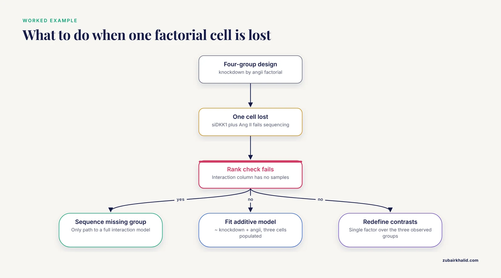
Consider the four-group structure from the Ang II study cited earlier, negative control, siDKK1, negative control with Ang II, and siDKK1 with Ang II [3], and imagine a lab ran the same design but lost the siDKK1-plus-Ang II group to a sequencing failure. The intended design is:
design <- ~ knockdown + angii + knockdown:angiiWith one cell empty, the interaction term includes a column for the missing combination that has no supporting samples, and the rank check fails. The cross-tabulation in Step 2 shows the zero cell immediately. Your options, in order of preference, are:
- Sequence the missing group. This is the only path to a full interaction model.
- Fit
~ knockdown + angiiwithout the interaction. This remains full rank with three cells populated and estimates additive effects, but it assumes the knockdown effect is the same with and without Ang II, which may be precisely the question the experiment was asking. - Redefine the contrast set around the three observed groups with a single four-level factor minus the missing level, using
results()contrasts between the groups that exist.
Option 2 and option 3 answer different questions than the original design, and the choice should be documented in the methods section rather than made silently in a script.
Common Mistakes and Limitations
Several specific mistakes recur in troubleshooting this error, and each one either wastes time or produces a worse analysis:
- Deleting covariates until the error stops. The first formula that runs is not the first formula that is correct. Every covariate you drop is a source of variation that now lands in the residual or, worse, in the coefficient of interest. Drop columns deliberately, in response to a diagnosed dependency, and record what you dropped and why.
- Treating the error as a count data problem. The error is purely a function of the design formula and colData. Your counts, your normalization, and your filtering are irrelevant to it. Debugging the count matrix for hours when the bug lives in a spreadsheet is the most common time sink in this troubleshooting session.
- Confusing partial with perfect confounding. A cross-tabulation with one or two off-diagonal samples still supports
~ batch + condition. Researchers sometimes drop the batch term in this situation and lose variance reduction they could have had. Check the rank numerically rather than eyeballing the table. - Adding blocking factors that do not block anything. A donor factor where each donor contributed one sample, or a site factor that mirrors the condition, consumes degrees of freedom and can trigger the error without adding estimable structure. The fibroblast study's finding that anatomic site, not donor, organized the samples [1] is a useful model for asking which metadata axis actually corresponds to independent units.
- Ignoring the interaction requirement. Interactions demand populated cells. Adding
:treatmentto a formula because it looks more complete is a frequent cause of the error in factorial experiments, including designs structured like the four-group Ang II study [3]. - Forgetting that DESeq2 has no random effects. Repeated measures with unbalanced structure, crossed random factors, and multi-level hierarchies exceed the formula syntax. Recognizing that boundary early, as studies that pair DESeq2 with other model frameworks do [9], saves a day of frustrated debugging.
- Overlooking general model assumption risk. Fixing the rank check makes the design estimable but does not by itself validate the model. Work on gene-set and pathway analysis demonstrates how violations of distributional assumptions propagate from the differential expression step into downstream interpretation [4], so treat the rank fix as one link in a chain of checks rather than the last one.
One limitation deserves plain language. When batch and condition are perfectly confounded, no fix exists, no software rescues the experiment, and the appropriate response is to report the limitation and, where the question matters, collect balanced data. Statistical tools recover information that the experiment contained. They cannot recover information the experiment never captured.
Prevention Practices
The rank error is almost always cheaper to prevent than to diagnose, because it is a design-time problem that surfaces at analysis time. Four practices cover nearly all of it.
Balance the batch structure at the experimental design stage. When planning the wet lab, allocate conditions across batches so every batch contains samples from every condition. Randomize library preparation order and sequencing lane assignment across conditions. Balanced batching makes ~ batch + condition full rank by construction and removes the most common failure mode entirely.
Curate one metadata table and freeze it. Build colData once, from a single source, with row names matching sample names exactly. Record batch, operator, library prep date, flow cell, sex, age, and every variable you might ever want to test. Store it as a versioned file. Most metadata assembly mistakes come from ad hoc merges in analysis scripts, and a frozen table eliminates them.
Dry-run the design matrix before the data arrive. You can build model.matrix(~ batch + condition, data = planned_coldata) from the sample sheet weeks before sequencing returns. Running qr()$rank == ncol(mm) at planning time catches confounding while there is still time to change the batch structure, which is the only moment when that fix is free.
Check the rank in the analysis script as an assertion. Make the check a permanent part of the pipeline so any future metadata edit that breaks the design fails fast with a clear message rather than a cryptic DESeq2 error two steps later:
stopifnot(limma::is.fullrank(model.matrix(design_formula, data = coldata)))The workflows that published successfully with DESeq2, across fibroblast sites [1], podocyte models [2], factorial cell stimulations [3], tumor response groups [7], dietary interventions [9], and carcinoma cohorts [6], [8], share this property: someone checked that the design matrix matched the experiment before trusting the coefficients. The "model matrix not full rank" error is DESeq2 insisting that you do the same.
Frequently Asked Questions
What does "model matrix not full rank" mean in plain language?
One of the columns in your design formula contains no information beyond what the other columns already provide, usually because two metadata variables tell the same story about your samples. DESeq2 cannot estimate a unique coefficient for redundant information, so it stops instead of returning an arbitrary answer.
Is this an RNA-seq error or a metadata error?
It is always a design and metadata error, never a count data error. Your counts, normalization, and filtering have no influence on the rank of the design matrix, so troubleshoot the sample sheet and the formula, not the expression matrix.
How do I find out which columns caused the failure?
Cross-tabulate the design factors with table() to spot confounding and empty cells, then run caret::findLinearCombos(model.matrix(...)) to name the exact redundant columns. The limma::nonEstimable() function gives a similar listing.
My batch and condition are perfectly confounded. Can DESeq2 still save the analysis?
No statistical method can separate two effects that were never varied independently in the experiment. Run ~ condition, report the confounding explicitly as a limitation, and treat the results as hypothesis-generating or re-plan the experiment with balanced batches.
Why does DESeq2 error when other tools seem to run the same design?
Some fitting functions silently drop redundant columns and report NA coefficients instead of stopping, which hides the problem rather than solving it. DESeq2 checks the rank at dataset construction and refuses, which protects you from fold changes whose meaning depends on which column the software happened to discard.
Should I include every metadata column in my design formula?
No. Include variables that represent real structure you want to adjust for or test, and require that blocking factors have samples repeated within their levels. Columns with one value per sample, derived totals, and percentage sets that sum to one will break the rank or waste degrees of freedom.
How many samples do I need in each group for the design to work?
Each coefficient in the design matrix needs at least one degree of freedom of support, which in practice means several biological replicates per condition and, for factorial designs, populated and reasonably replicated cells for every combination of factor levels. Three biological replicates per group is the conventional minimum, and more is better for interaction testing.
Can DESeq2 handle paired or repeated-measures RNA-seq data?
Yes for balanced paired designs, using a blocking factor such as ~ patient + treatment, where every patient contributed samples to every condition. For unbalanced repeated measures or designs needing random effects, DESeq2's formula syntax cannot express the model, and limma-voom with duplicateCorrelation or a linear mixed model tool is the appropriate alternative.
Sources
- Tissue specific human fibroblast differential expression based on RNAsequencing analysis.
- Genome-wide expression analysis in a Fabry disease human podocyte cell line.
- DKK1/SMDT1 participate in Ang II-induced mitochondrial injury of human smooth muscle cells in an abdominal aortic aneurysm cell model.
- The impact of distributional assumptions in gene-set and pathway analysis: how far can it go wrong?
- Critical Differential Expression Assessment for Individual Bulk RNA-Seq Projects
- A Comprehensive Analysis of Novel Variations Associated with Bile Duct Cancer: Insights into Expression, Methylation, and 3D Protein Structure.
- Pilot study on differential gene expression in relation to vincristine response in canine transmissible venereal tumor.
- Prognostic and therapeutic implications of extracellular matrix associated gene signature in renal clear cell carcinoma.
- Fiber deprivation and insoluble corn-based fibrous -co-products modulate gastrointestinal mucosa-associated microbiota, extracellular matrix remodeling, and intestinal morphology in growing pigs.