How to Interpret DESeq2's 'LFC Shrinkage' Results

By Dr. Zubair Khalid, DVM, MS, PhD · 2026-11-11

In DESeq2, LFC shrinkage replaces each gene's raw maximum likelihood estimate of the log2 fold change with an empirical Bayes posterior estimate that is pulled toward zero by an amount determined by the gene's counts and the overall evidence in the dataset. The shrunken log2FoldChange is a more stable effect size for ranking, visualization, and filtering, while the p-value and adjusted p-value from the Wald test remain unchanged.

This distinction matters because the raw fold change and the shrunken fold change answer different questions. The raw estimate answers, "what fold change does this gene's count data alone suggest?" The shrunken estimate answers, "given what the whole experiment tells us about how noisy low-count genes are, what fold change is most plausible for this gene?" Confusing the two is one of the most frequent causes of an RNA seq error in differential expression reporting, and it shows up in two opposite ways. Genes with tiny counts but dramatic raw fold changes get overinterpreted, and genes with solid evidence get their honest effect sizes obscured in tables built from raw estimates. This article gives you the DESeq2 LFC shrinkage interpretation you need to read a results table, choose a shrinkage estimator, and explain the numbers to a collaborator without hedging.

What LFC Shrinkage Means in DESeq2

LFC stands for log2 fold change. For a gene with a mean expression of 100 counts in control and 400 counts in treated, the fold change is 4 and the log2 fold change is 2. Negative values mean the gene is lower in the treated group. DESeq2 fits a negative binomial generalized linear model to each gene's counts, and the coefficient for the condition term in that model is the log2 fold change.

Without shrinkage, the coefficient reported by results() is the maximum likelihood estimate (MLE), the value of the coefficient that makes the observed counts most probable under the fitted model. With shrinkage, lfcShrink() combines that likelihood with a prior distribution on fold changes, centered at zero, whose width is estimated from the data itself. The reported number becomes a posterior estimate, usually the posterior mean or mode. Because the prior pulls every estimate toward zero, and pulls hardest where the data provide the least information, the practical effect is that noisy, low-count, extreme fold changes shrink a lot and well-supported fold changes shrink very little.

A useful mental model: shrinkage is a data-driven skepticism filter for effect sizes. It does not ask whether a gene is differentially expressed. The Wald test already did that. It asks how large the effect probably is, given that extreme fold changes from weakly expressed genes are usually artifacts of small counts.

Why DESeq2 Shrinks Fold Changes

Three problems in RNA-seq data motivate the method, and all three trace back to the same statistical fact. For a low-count gene, say a gene with counts of 1, 0, 2 in one group and 0, 1, 0 in the other, the log2 fold change estimate is unstable. A single extra read can move the estimate by several log2 units. The standard error reflects this instability, but the raw point estimate itself sits at some absurd value like log2(3/0.5), and anything you do downstream that sorts by fold change will put that gene at the top of the list.

The first problem is ranking. Tables sorted by raw absolute log2 fold change are dominated by genes with counts near zero. These genes are typically the least biologically interesting and the least reproducible. Reviews of differential expression practice emphasize that ranking behavior differs across tools and that method choice, including how effect sizes are estimated and regularized, directly affects which genes surface at the top of a candidate list [1].

The second problem is visualization. An MA plot of raw estimates shows a funnel of extreme points at low expression that carries no meaning. Shrunken estimates collapse that funnel, so the plot shows the structure you actually want to see, namely which genes have both significance and effect size.

The third problem is interpretability. If you tell a collaborator that a transcription factor is "20-fold upregulated" and the number came from a gene with counts of 2 versus 0, you have communicated something false. A shrunken estimate, or at minimum an honest look at the counts, prevents that. Methods comparisons for individual bulk RNA-seq projects, including work that tests GLM-based differential expression tools with robust dispersion estimation against known causal genes, show that the details of the statistical pipeline, not just the p-value cutoff, determine whether the gene you care about actually ranks where you need it [1].

One more motivation deserves mention because it is easy to overlook. Standard differential expression analysis assumes that the composition of the RNA pool is roughly comparable across samples. When master regulators such as c-MYC shift expression globally, that assumption breaks, and systematic studies show that some differential expression methods tolerate the resulting global shift better than others while classification and downstream conclusions can be biased [2]. Shrinkage does not fix compositional bias, but shrunken effect sizes are less likely to amplify it, because the most extreme raw estimates, which are often the ones most entangled with composition artifacts, get moderated first.

How the Shrinkage Mechanism Works, Step by Step

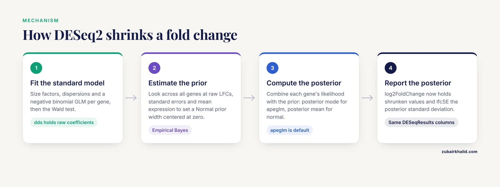
Understanding the mechanism answers most "what does deseq2 lfc shrinkage interpretation mean" questions before they arise. The process has four steps.

Step 1. Fit the standard model. DESeq2 estimates size factors (sequencing depth correction), gene-wise dispersions, and fitted dispersions, then fits a negative binomial GLM per gene and runs the Wald test. At this point the DESeqDataSet object dds holds both the raw coefficients and their standard errors.

Step 2. Estimate the prior. DESeq2 looks across all genes at the relationship between the raw log2 fold changes, their standard errors, and mean expression. From this it estimates the width of a Normal prior on the coefficients, centered at zero. Genes with high counts and low dispersion drive the prior to be wide, which means the prior tolerates large fold changes when the data generally support them. Genes with weak evidence pull the prior narrower. This is what makes the procedure empirical Bayes, the prior comes from your data, not from a fixed external setting.

Step 3. Compute the posterior. For each gene, lfcShrink() combines the likelihood from the GLM with the prior and reports the posterior estimate. For the apeglm method, the default since DESeq2 version 1.28, this is the posterior mode computed with the apeglm package. For the older "normal" type it is the posterior mean. For ashr it is based on the adaptive shrinkage framework that models effects as coming from a mixture of point masses and scales.

Step 4. Report the posterior in place of the MLE. The object returned by lfcShrink() is still a DESeqResults object with the same columns as before, but the log2FoldChange column now holds shrunken values and lfcSE holds the corresponding posterior standard deviation rather than the Wald standard error.

The key behavioral pattern to internalize: shrinkage is a function of information. A gene with mean normalized counts of 5,000 and a raw LFC of 1.8 will barely move, perhaps to 1.78. A gene with mean counts of 12 and a raw LFC of 6.5 can shrink to 1.1. Both moves are correct. The first gene's estimate was already well supported. The second gene's estimate was mostly noise, and the prior knew that from the genome-wide pattern.

The Shrinkage Estimators and When to Use Each

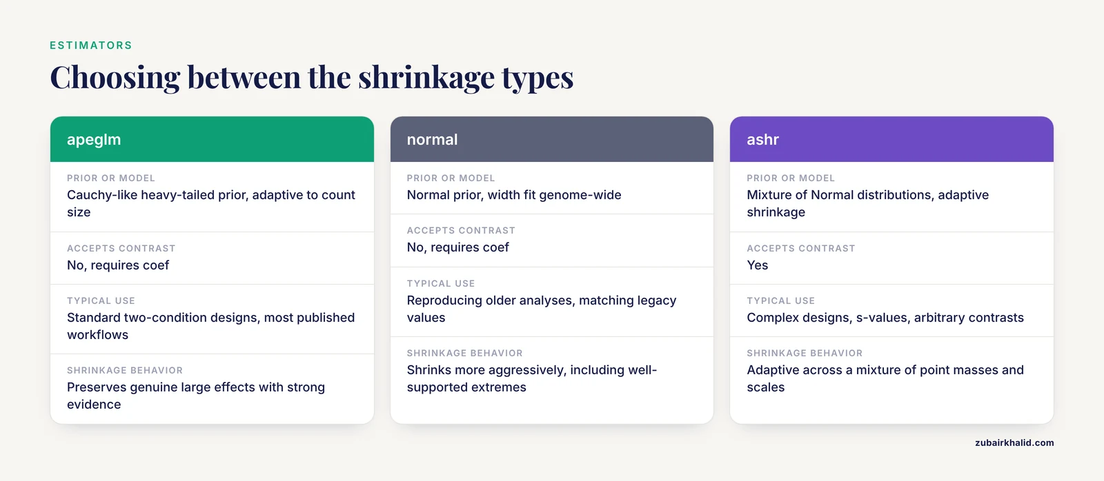
DESeq2 offers several shrinkage types through the type argument of lfcShrink(). They differ in the prior they use, whether they can be applied to arbitrary contrasts, and what they return.

Three practical consequences follow from this table.

First, the choice of type changes the numbers but rarely changes which genes are significant. If a collaborator asks whether switching from normal to apeglm will change the DE gene list, the answer is usually no, because p-values and adjusted p-values carry over.

Second, apeglm requires coef rather than contrast. You must run resultsNames(dds) first and pick the coefficient string, for example "condition_treated_vs_control". If your comparison is not in the results names, either relevel the factor or use ashr, which accepts a contrast argument directly.

Third, heavy-tailed priors like apeglm's shrink less aggressively for genes that genuinely show extreme effects with strong evidence, which is why apeglm became the default. Under a thin-tailed Normal prior, a truly dramatic, well-supported 32-fold change gets squeezed more than most biologists find comfortable.

Running lfcShrink: A Complete R Workflow

The workflow below shows the exact sequence and where shrinkage enters. This is the standard pattern documented in the DESeq2 vignette and used across published pipelines, and tools that wrap RNA-seq analysis into accessible interfaces, such as BioWardrobe, expose the same differential expression logic with built-in quality control steps so that users can troubleshoot the upstream experiment as well as the statistics [3].

library(DESeq2)

# Standard pipeline through the Wald test
dds <- DESeqDataSetFromMatrix(countData = cts,
                              colData   = coldata,
                              design    = ~ condition)
dds <- DESeq(dds)

# What coefficients exist?
resultsNames(dds)
# [4] "Intercept"  "condition_treated_vs_control"

# Raw (unshrunken) results
resRaw <- results(dds, alpha = 0.05)

# Shrunken results, apeglm (default since DESeq2 1.28)
resShrunk <- lfcShrink(dds, coef = "condition_treated_vs_control",
                       type = "apeglm", res = resShrunk)

A common error appears in that last line. When you pass res to lfcShrink() with type apeglm, pass the shrunken object itself as the target, or omit res entirely and DESeq2 will run results() for you with default settings. If you pass a res object that was created with a different contrast than coef, the function will warn you, and you should take the warning seriously because it means the fold change in your table may not correspond to the comparison you intended.

For a contrast that is not a single coefficient, for example a difference between two treated groups relative to control in a three-level design, use ashr.

resAsh <- lfcShrink(dds, contrast = c("condition", "treatedA", "treatedB"),
                    type = "ashr", res = resAsh)

Two diagnostic plots belong in every analysis. The first is the MA plot, which DESeq2 renders with shrunken estimates automatically when the input is a shrunken DESeqResults object.

plotMA(resShrunk, alpha = 0.05, main = "Shrunken LFC, apeglm")

Compare it against plotMA(resRaw) and you will see the signature of shrinkage, a collapse of the scattered extreme points at the low-expression end of the x-axis into a band near zero, while high-expression genes hold their positions. The second is a simple check on the genes whose fold changes moved the most.

idx <- order(abs(resRaw$log2FoldChange), decreasing = TRUE)[1:20]
data.frame(raw = resRaw$log2FoldChange[idx],
           shrunk = resShrunk$log2FoldChange[idx],
           baseMean = resShrunk$baseMean[idx])

In almost every real dataset, that table tells the whole story. The genes with the largest raw LFCs and the smallest baseMeans are the ones that shrink the hardest, and seeing it with your own gene names is worth more than any abstract explanation.

Reading the Shrunken Output Column by Column

The DESeqResults object from lfcShrink() contains the same six columns as a standard results() output, but two of them mean something different after shrinkage.

baseMean. Unchanged. The mean of normalized counts across all samples. This is your anchor for judging how much shrinkage likely affected a gene, because high baseMean genes were barely touched.

log2FoldChange. Now the posterior estimate, not the MLE. This is the number to report, rank on, and plot.

lfcSE. After shrinkage with apeglm or ashr, this is the posterior standard deviation, not the Wald standard error. It is generally a bit larger than the Wald SE for low-count genes, which is the honest reflection of uncertainty under the prior. Do not use this column to recompute z-scores and p-values, that reconstruction is not valid and reproduces nothing.

stat, pvalue, padj. Carried over from the Wald test. For the default shrinkage types these columns are identical to what results() produced. Shrinkage is a statement about effect size estimation, not about hypothesis testing. If you see p-values change after switching shrinkage types, something is wrong in your code, most often a mismatch between coef and the res object you passed in.

A fifth quantity, the s-value, appears only when you request it with type ashr. The s-value is a quantity related to the false sign rate. An s-value of 0.01 means that the collection of genes with s-values at or below 0.01 has at most about a 1 percent chance of containing genes whose shrunken fold change has the wrong sign. S-values answer a question that p-values were never designed to answer, namely how confident you can be in the direction and rough magnitude of the effect rather than merely in the existence of some difference.

Interpreting Shrunken LFCs in Practice

Here is an illustrative example with realistic numbers. Suppose your dataset has six samples, three control and three treated, and you are looking at two genes.

Gene A has baseMean 4,200, raw LFC 1.75, Wald SE 0.11, p-value 2e-9. After apeglm shrinkage, LFC 1.74. Almost nothing happened because the counts are high, the dispersion is low, and the evidence is overwhelming. Report the shrunken value, which corresponds to roughly a 3.3-fold change, and you are on solid ground.

Gene B has baseMean 9, counts of 0, 1, 2 in control and 8, 14, 22 in treated, raw LFC 4.6, Wald SE 1.2, p-value 0.021, adjusted p-value 0.14. After shrinkage, LFC 1.9. The raw estimate claimed a 24-fold induction. The shrunken estimate claims roughly a 3.7-fold induction, and both p-values tell you this gene does not survive multiple testing correction anyway. If you had sorted by raw LFC and built a figure around Gene B, the shrinkage output just saved you from a retraction-grade misstatement.

Now the harder case. Gene C has baseMean 15, counts of 0, 0, 1 in control and 12, 18, 25 in treated, raw LFC 6.2, p-value 1e-4, adjusted p-value 0.02. Shrinkage pulls it to 3.1. This is the case that generates the most questions. The gene is genuinely significant, the counts are consistent, and yet the fold change was cut in half. The interpretation is that the direction and the significance are trustworthy, the magnitude estimate from eleven total reads was not. The gene may well be strongly induced. Shrinkage is telling you that the data support "at least a few-fold induction with high confidence" more than they support "64-fold induction." If the precise magnitude matters for your conclusion, the fix is more sequencing depth or more replicates, not a different shrinkage setting.

For fold-change filtering, DESeq2's lfcThreshold argument in results() deserves a separate note because it is frequently confused with shrinkage. results(dds, lfcThreshold = 1) performs a Wald test of the null hypothesis that the true LFC is between -1 and 1. It changes the test, not the estimate. Shrinkage changes the estimate, not the test. Publications that predefine effect-size criteria, for example requiring a fold change above 1.5 alongside an FDR cutoff, are combining an effect-size threshold with a significance threshold, and the shrunken LFC is the right quantity to apply such thresholds to [1].

Downstream Uses: Ranking, Volcano Plots, and Gene-Set Analysis

Where should shrunken values flow downstream, and where should they not?

For ranking and candidate prioritization, use shrunken values without hesitation. Combined rankings that sort on a product or weighted sum of significance and effect size behave far better with shrunken LFCs because the low-count extremes no longer distort the ordering. This matters for the kind of project-level decision making described in work on critical differential expression assessment, where the goal is to make sure a known causal gene is recovered rather than buried by noisy candidates [1].

For volcano plots, plot shrunken LFC on the x-axis. The plot becomes interpretable, because the points that stretch the x-axis are genes with both evidence and effect, not artifacts of a single read.

For gene-set and pathway analysis, the situation is more subtle, and this is where a genuine statistical caution applies. Many gene-set analysis methods rest on distributional assumptions about the input scores, and systematic work testing those assumptions across tumor and normal datasets found that the multivariate normal assumption behind some parametric gene-set methods is often violated, which degrades performance in ways that depend on the method [4]. When you feed shrunken LFCs into a competitive gene-set test such as a rank-based method, the shrinkage changes the shape of the score distribution, typically by compressing the tails. Ranking-based methods such as those in the fgsea family are comparatively robust to this, but parametric tests that assume the input scores follow a specific distribution can shift their calibration. The practical rule is to keep the input to gene-set analysis consistent across the genes you compare, always shrunken or always raw, and to prefer rank-based methods when in doubt, because their performance under non-normal input has been examined directly [4].

For single-cell extensions, the same logic carries over with one modification. In scRNA-seq, the sparse count structure makes raw fold changes even less stable than in bulk, and modern single-cell protocols stress careful parameter selection and structured troubleshooting across preprocessing, integration, and differential expression steps for exactly this reason [5]. When differential expression on single-cell data is run through a pseudobulk DESeq2 pipeline, apply the same shrinkage interpretation described here to the aggregated counts.

Bioinformatics Troubleshooting: When Shrunken Results Look Wrong

Most complaints about shrinkage fall into a small set of recurring patterns, and each has a specific diagnosis. This section doubles as a general RNA seq error checklist for the shrinkage stage of a pipeline.

Pattern 1. All my fold changes got smaller and a collaborator is unhappy. This is expected behavior, especially with the normal-type prior on a dataset with many weakly expressed genes. Reassure with the MA plot comparison. If the shrinkage feels too aggressive for well-supported genes, switch to apeglm, which uses a heavier-tailed prior and preserves extreme but genuine effects better.

Pattern 2. lfcShrink returns an error about coef. You passed a contrast to coef, or the coefficient name has a typo. Run resultsNames(dds) and copy the exact string. If you need a custom contrast, use type = "ashr".

Pattern 3. Warning about res and coef mismatch. You built res with one comparison and are shrinking another. Regenerate res with the matching contrast, or drop the res argument.

Pattern 4. Shrunken LFCs are still enormous for near-zero genes. Check your size factors. If one sample has a size factor far from 1, or if you skipped normalization entirely, the model input is broken and no shrinkage setting will rescue it. This is an upstream QC problem of the kind that interface-based RNA-seq tools attempt to catch with automated quality measures, and the fix lives in the count matrix and metadata, not in lfcShrink() [3].

Pattern 5. Results disagree between DESeq2 and another tool such as edgeR. Partial disagreement is normal, because the tools differ in dispersion estimation and in how they handle effect sizes. EdgeR's quasi-likelihood pipeline with robust dispersion estimation can recover a known causal gene in settings where other parameterizations miss it, which is why method-conscious projects sometimes run two tools and prioritize genes called by both [1]. Shrunken LFCs from DESeq2 are usually closer to edgeR's moderated estimates than raw DESeq2 LFCs are, because both apply a form of information borrowing.

Pattern 6. Everything looks fine statistically but the biology does not validate. Before blaming shrinkage, check the assumptions the whole analysis rests on. A global expression shift, common when a master regulator is perturbed or when comparing tumor and normal tissue, violates the assumption that the total RNA pool is comparable across samples and can bias differential expression results and classification in ways that vary by method [2]. Also remember that mRNA abundance is not protein abundance, and critiques of large-scale expression analyses explicitly recommend checking protein-level evidence, for example through reverse-phase protein array resources, before building conclusions on transcript fold changes alone.

Pattern 7. padj is NA for genes with tiny p-values. Independent filtering removed them because their mean normalized counts fall below a threshold where the test has no power. Shrinkage will still produce an LFC for these genes, but the filtered genes should not enter ranked lists as significant hits.

Common Mistakes and Limitations

Mistake 1. Treating the shrunken LFC as a new statistical test. Shrinkage changes the effect size estimate. It does not create, destroy, or modify p-values under the default settings. Reporting "shrunken p-values" is a category error.

Mistake 2. Reconstructing p-values from shrunken LFC and lfcSE. Dividing the shrunken LFC by the posterior lfcSE and treating the result as a z-statistic is not valid. The posterior quantities do not combine into a Wald statistic.

Mistake 3. Reporting fold changes as "X-fold" without checking direction and base. A shrunken LFC of -2 is a 4-fold decrease, not a 2-fold change. Always antilog with sign awareness, and always report which group is the numerator.

Mistake 4. Using raw LFCs for filtering and shrunken LFCs for plotting in the same project. Pick one convention, document it, and apply it everywhere. Mixed conventions produce tables and figures that contradict each other.

Mistake 5. Assuming shrinkage fixes compositional bias. Shrinkage moderates per-gene effect estimates. It does not correct a global shift in the RNA content of one condition, which can bias both DE detection and molecular classification in method-dependent ways [2].

Mistake 6. Assuming shrinkage fixes normalization or batch problems. If the design formula omits a known batch variable, or if size factors are distorted, the shrunken estimates inherit the problem. Troubleshoot upstream.

Limitation 1. Shrinkage is not independent validation. A stable effect size estimate is not the same as replication in an independent cohort. Cross-database and cross-platform validation strengthen conclusions from expression profiling, and restricting an analysis to a single data source can bias results in ways that change the conclusion.

Limitation 2. Shrunken LFCs depend on the whole dataset. Adding or removing samples changes the prior width, so shrunken values from one version of an analysis are not exactly reproducible in another with different sample composition. Raw MLEs are more stable under sample-set changes, which is occasionally a reason to report them, for example when pooling results across independent studies.

Limitation 3. Transcript-level vs protein-level inference. A shrunken LFC describes RNA abundance. Whether that translates to protein and function depends on biology the model does not see, and expression-based conclusions benefit from protein-level follow-up where available.

Quick Review

• LFC shrinkage converts the raw maximum likelihood log2 fold change into an empirical Bayes posterior estimate, pulled toward zero in proportion to how little information supports the gene.
• Significance does not change. p-value and adjusted p-value carry over from the Wald test unchanged under the default shrinkage types.
• Low-count genes shrink the most, high-count genes barely move. Check baseMean when you are surprised by a shrinkage amount.
• apeglm is the default and requires coef. ashr accepts contrast and is the route to s-values.
• lfcSE in a shrunken object is a posterior standard deviation, not a Wald SE, and cannot be used to recompute p-values.
• Use shrunken LFCs for ranking, volcano plots, and fold-change filters. Use rank-based gene-set methods and keep the score convention consistent across analyses.
• Shrinkage does not correct compositional bias, batch effects, or normalization failures, and it is not a substitute for independent validation.

Frequently Asked Questions

Does LFC shrinkage change p-values or adjusted p-values?

No. Under the default shrinkage types, the pvalue and padj columns are carried over from the standard Wald test unchanged. Shrinkage replaces only the effect size estimate, and if your p-values appear to change after adding shrinkage, check for a mismatch between the coef argument and the res object you passed to lfcShrink().

Should I use coef or contrast in lfcShrink?

Use coef with the default apeglm and normal types, taking the exact string from resultsNames(dds). Use contrast only with type = "ashr", which is also the right choice for comparisons that are not a single model coefficient, such as differences between two treatment levels relative to a shared control.

Which shrinkage type should I choose, apeglm or ashr?

For a standard two-condition comparison, use apeglm, the DESeq2 default, because its heavy-tailed prior preserves genuine large effects with strong evidence while still moderating low-count noise. Choose ashr when you need to shrink a custom contrast or when you want s-values as a false-sign-rate-aware alternative to adjusted p-values.

Why did my large fold change shrink to almost zero?

The gene probably has very low counts, and the raw LFC was driven by one or two reads, so the prior correctly judged the magnitude to be unsupported. Check the baseMean column and the raw per-sample counts. If the effect is real and the magnitude matters, the solution is greater sequencing depth or more replicates.

Can I use shrunken log2FoldChange values for GSEA?

Yes, and they are usually the better input for rank-based gene-set methods, because they remove low-count extremes that otherwise dominate sorted lists. Keep the score convention consistent across all genes and runs, and prefer rank-based methods over parametric ones, since parametric gene-set tests are sensitive to distributional assumptions that shrunken scores do not satisfy in a predictable way.

What does an s-value mean?

An s-value bounds the rate of false sign statements. Genes with s-values at or below 0.01 are a set for which at most about 1 percent are expected to have shrunken fold changes pointing in the wrong direction. The s-value is available with type = "ashr" and answers a question about effect size direction and magnitude that p-values were not designed to address.

Sources

1. Critical Differential Expression Assessment for Individual Bulk RNA-Seq Projects
2. The Influence of the Global Gene Expression Shift on Downstream Analyses
3. Analysis of ChIP-Seq and RNA-Seq Data with BioWardrobe
4. The impact of distributional assumptions in gene-set and pathway analysis: how far can it go wrong?
5. A Reproducible Seurat-Based Protocol for Single-Cell RNA Sequencing Analysis of Peripheral Blood Mononuclear Cell CD4+ T Cells During Malaria Reinfection.